How to Use COUNTUNIQUE function in Google Sheets

The COUNTUNIQUE function in Google Sheets counts the number of unique values in a dataset.

It is especially useful when you want to sort through large amounts of data.

The rules for the COUNTUNIQUE function in Google Sheets are:

• The COUNTUNIQUE function is applicable to any kind of data, numerical or nominal.
• It is a variation of the COUNT function that counts only unique data, regardless of how many times they are repeated in a dataset.

Consider this example.

You’re a financial advisor of insurance and investment plans. You’ve helped numerous clients throughout the year, and you want to give them a little Christmas present. Now, some of your clients have only one investment plan, but some others have more than one. Your database is also sorted according to policy numbers rather than client names. How can you tell exactly how many clients you have? 

The COUNTUNIQUE function can find that information for you. You might be able to manually count the number of unique values in a smaller database, but sometimes, the values in your database can number over the thousands. In those cases, manually counting for unique values leaves a lot of room for error. The COUNTUNIQUE function can tell you how many unique values you have more accurately and with less effort. 

It’s easy to learn and gets the job done. ✅

That’s one example where learning the COUNTUNIQUE function in Google Sheets can be valuable, and there are many more. For instance, In a library catalog, you can use it to know how many titles you have rather than how many books. 

Whatever the purpose, the COUNTUNIQUE function gives you accurate information for less work.

Great! Let’s see how it’s used in a more detailed example. We’ll work with an actual database and find all the unique values. It will also help us correctly write our own COUNTUNIQUE functions in Google Sheets. As COUNTUNIQUE is a variation of the COUNT function, we’ll also illustrate how their results can differ.

The Anatomy of the COUNTUNIQUE Function

So the syntax (the way we write) of the COUNTUNIQUE function is as follows:

=COUNTUNIQUE(value1, [value2, …])

Let’s go through each part of the function and understand what each term mean:

• = the equal sign is always how we start any function in Google Sheets.
• COUNTUNIQUE() is our COUNTUNIQUE function. It will analyze the data written in the function and return the number of unique values in finds. 
• Value is any data you want to consider for uniqueness. This can be written into the function, a cell, a range of cells, or a combination of all three. At least one value is required to perform the function. All other values are optional.

A Real Example of Using the COUNTUNIQUE Function

How can you apply this in real life? Check out this example below to see how COUNTUNIQUE is used in Google Sheets. 

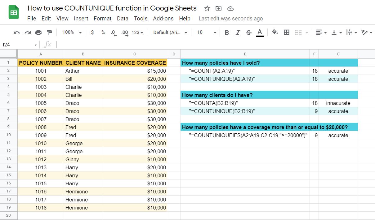
Let’s expound on the example from above. You’re a financial advisor, and the image above is a simplified version of your database. It shows all the policies you’ve sold and their respective clients. Christmas is coming and you want to give each client a little present. How many presents do you prepare?

You wouldn’t want to refer to the number of policies, as some clients have more than one, and would, therefore, receive more than one present. You’ll want to refer to your CLIENT NAME dataset and use the COUNTUNIQUE function to count all the unique client names. Then you’ll know how many clients you have and how many presents to prepare.

As you can see in the example, the COUNTUNIQUE function returns a number of 9 unique values from the CLIENT NAME column. The COUNTA function, on the other hand, which returns the number of all values regardless of uniqueness, gives a number of 18. 

In this situation, the COUNTUNIQUE is the right function for your purpose. 

You may make a copy of the spreadsheet using the link I have attached below. 

There is also another variation of the COUNTUNIQUE function called the COUNTUNIQUEIF. This function combines the COUNTUNIQUE and IF functions to result in the counting of conditional values. 

For example, you want to know how many policies you’ve sold have insurance coverage of more than or equal to $20,000. The COUNTUNIQUE function counts the number of unique values in a range, filtered by a set of criteria applied to additional ranges. If you count it manually, there are 9 policies with a coverage of $20,000 or more, which is the same result as the COUNTUNIQUEIFS but without the hassle.  

I will write a more advanced tutorial on how you can use the COUNTUNIQUEIFS function with other functions in the coming weeks. Be sure to subscribe through the form below to be notified. 

Now let’s begin writing our own COUNTUNIQUE function in Google Sheets.

How to Use COUNTUNIQUE Function in Google Sheets

1. Firstly, prepare the data you want to use. To help illustrate the effect of the COUNTUNIQUE function, it would help if some data are repeated. If you don’t have a ready database to use, feel free to make a copy of this one. 

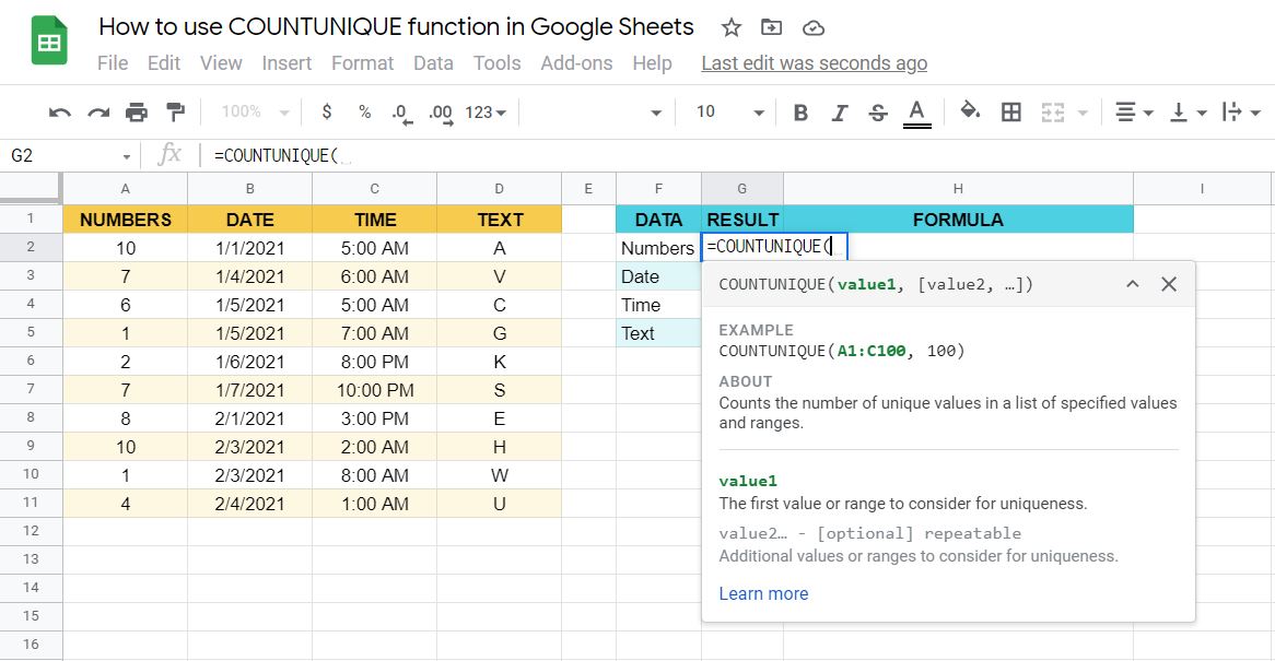
2. Next, click on any cell you want to use. Any cell will do. This is where the result will appear. Type in the equal sign ‘=‘ to open the function. Follow that by the name of the function which is ‘countunique‘ (or ‘COUNTUNIQUE‘, either one will work).

3. The auto-suggest box will appear with the names of the functions that start with COUNTUNIQUE. At the moment, there are only two – COUNTUNIQUE and COUNTUNIQUEIFS. We’ll cover the latter in a separate tutorial. For now, select COUNTUNIQUEby pressing the Tab or Enter keys on your keyboard. A guide from Google Sheets will appear that tells you more about the function you’re using. Click on this ^ symbol on the upper right of the box beside the x, to minimize the box.

4. The next step is to put in the values. This can be anything. You can put a set of numbers (as shown below), a range of cells, or both. To end the function, type in a close parenthesis.

5. Now, hit your Enter key on your keyboard. The result should appear in the cell you used for the function. For this example, the count of unique number values is 7.

6. Let’s have another example! This time, let’s find the number of unique Date values. Select a range of cells to input the values. This method of inputting value is more efficient and accurate. To do that, click on the first cell in the range and drag your mouse to the last cell. You can also just type it in as B2:B11, B2 is the first cell, and B11 is the last cell.

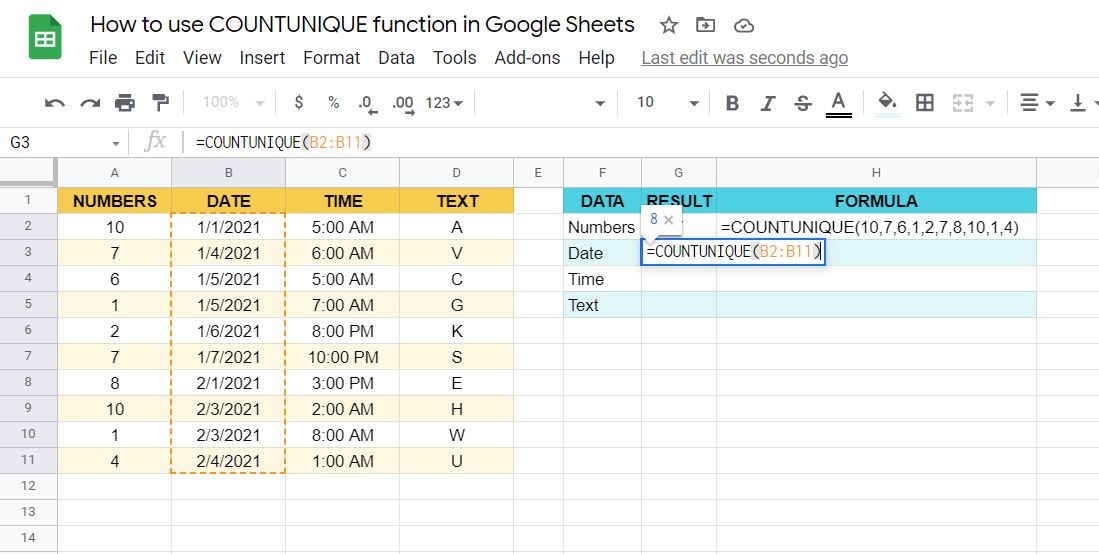
7. To execute the function, press the Enter key on your keyboard. In this example, there are eight unique values in the Dates dataset.

8. Just repeat steps 6 and 7 on the remaining two datasets. You should have the same results below.  

And that’s the end of this tutorial. You can now use the COUNTUNIQUE function in Google Sheets to find the number of unique values in any dataset. Combine it with other Google Sheets functions for more powerful and effective formulas that improve efficiency and accuracy in your work. 

Get emails from us about Google Sheets.

Our goal this year is to create lots of rich, bite-sized tutorials for Google Sheets users like you. If you liked this one, you'll love what we are working on! Readers receive ✨ early access ✨ to new content.

Subscribe