


To find the last value in each row in Google Sheet using the LOOKUP function is useful if you want to extract the last used column in your data set.
Table of Contents
Let’s take an example.
Say we have some rooms in a school and we keep track of the students who used these rooms for their activities. We want to easily see who was the last person using each room.
So how do we do that?
Easy. We need to find the last non-empty cell in each row.
The LOOKUP function helps us do that. It searches through a row or column for a key value and then returns the value of the cell in a result range located in the same position as the search row or column. You will gain a better understanding after a couple of examples. 🙂
Let’s dive into the examples to show you how we can write our own LOOKUP function in Google Sheets to find the last non-empty cell in each row.
The Anatomy of the LOOKUP Function
The syntax (the way we write) the LOOKUP function is as follows:
=LOOKUP(search_key, search_range|search_result_array, [result_range])
Let’s dissect this thing so we’d better understand what each term means:
=the equal sign is how we start any function in Google Sheets.LOOKUPis our function. We will have to add the arguments into it to make it work.search_keyis the value to search for in the selected row or column.search_range|search_result_arraymeans that we have two options to choose from.- The first option is to use
search_rangeandresult_range(the third argument) together. In this situation, we search for the key in thesearch_rangeand we get output values fromresult_range. - The second option is to ignore
result_rangeand only usesearch_result_array, where the formula searches the first row or column and returns the value from the last row or column in the array. result_rangeis the range of cells from which the formula returns a result. The value returned corresponds to the location wheresearch_keyis found insearch_range. It should not be used if using thesearch_result_arraymethod.
The Behaviour of LOOKUP Function
To explain, let’s see closely how the LOOKUP function actually works.
For example, look at this example where
search_keyis 3,search_rangehere is an array containing numbers from 1 to 4,result_rangeis another array containing text values from “a” to “d”.
=LOOKUP(3, {1,2,3,4}, {"a","b","c","d"})
The function searched for the value 3 in the array of numbers, finds the number 3, and returns the corresponding value from the result range. So the result is “c”.
If there are more than one matching values, the function always returns the last one that matches the search_key. Look at this function:
=LOOKUP(3, {1,2,3,3,3,4}, {"a","b","c","d","e","f"})
This function returns the corresponding value of the last found 3 value, which is the letter “e” in this example. Eventually, this behavior is what we are going to use to find the last value in each row!
But that’s not all. Let’s have a look at the case when none of the cells matches the search_key.
=LOOKUP(8, {1,2,3,3,3,4}, {"a","b","c","d","e","f"})
This function tries to look up the value 8 in the second array. However, there is no 8 in this range. In this case, the LOOKUP function searches for the immediately smallest value of the range, which is number 4 in this example. It returns the corresponding value of 4, which is “f” in this example.
A Real Example of Using LOOKUP Function
Look at the example below to see how LOOKUP function is used to find the last value in each row in Google Sheets.

Option #1: LOOKUP with a text value that is surely the largest value
=LOOKUP("zzz", B2:E2)
Here’s what this example does:
- We wrote a
LOOKUPfunction with two arguments separated by commas in row 2. - In fact, we use the behavior mentioned above when none of the cells in the range matches the search key.
- We created a
search_key“zzz” that is definitely later in a sorted list than any of our actual values (students’ names). - We add the
search_result_arraywhich is the whole row we are working on (row 2 in the example containing the cells between B2:E2). - Finally, we drag-down the function to apply it to the other rows of the data set as well.
Option #2: LOOKUP by converting the text values into numbers
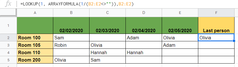
=LOOKUP(1, ARRAYFORMULA(1/(B2:E2<>"")),B2:E2)
Here’s what this example does:
- We wrote a
LOOKUPfunction with three arguments separated by commas in row 2. - In this example, we match the content of the cells with numbers so that we can use the
LOOKUPfunction with numbers instead of strings. This way, we don’t have to use a burnt-in “zzz” value but instead, create a more secure solution using numbers. - We work within a range of a row, so we use the B2:E2 range as the
result_rangeand also inside thesearch_range, but this one needs some modification in order to work with numbers. - Firstly, look at the second argument, which is an
ARRAYFORMULAfunction. We use this to match the content of the cells with numbers. TheARRAYFORMULAat the beginning of this argument ensures that we work with an array (the whole row) and not just with one cell. - Inside the brackets, there is the B4:E4<>”” expression. The <> operator means “not equal” and the “” (double quotes) means empty content since nothing is between the quotes. So this part of the formula checks whether a cell in a range is empty or not.
- Now let’s explain why there is a division (1 / B4:E4<>””). In short, it’s needed to convert boolean values into numbers. The expression B4:E4<>”” returns either TRUE or FALSE. When we divide 1 by a cell containing TRUE value, we get 1 as a result because TRUE is considered as a 1 in Google Sheets. Similarly, when we divide 1 by FALSE (considered as a 0 in Google Sheets), we get a division error because we tried to divide by 0. In conclusion, when the cell is not empty, we get a 1. When the cell is empty, we get an error which is not a number, so we excluded these cells from our LOOKUP search.
- Now we need to find the last cell that matches the
search_key. We put 1 as thesearch_keybecause we are looking for those non-empty cells. The LOOKUP function searches for thesearch_key, and as we have seen above, it gives the last cell in the array that has the value 1. - The
result_rangecontains the actual names, so the result of the whole function is the content of the last cell that is not empty. Great! We needed exactly that name. - Finally, we drag-down the function to apply it to the other rows of the data set as well.
Try it out by yourself. You may make a copy of the spreadsheet using the link I have attached below and try it for yourself:
How to Find Last Value in Each Row in Google Sheets
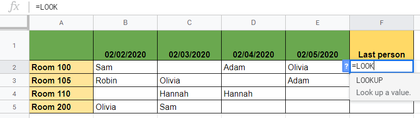
- To start, simply click on a cell to make it the active cell. For this guide, I will be selecting F2, where I want to show my result of row 2.

- Next, type the equal sign ‘=’ to begin the function and then followed by the name of the function which is ‘
lookup‘ (or ‘LOOKUP‘, whichever works).
- Great! You should now find that the auto-suggest box will pop-up with the name of the function
LOOKUP.
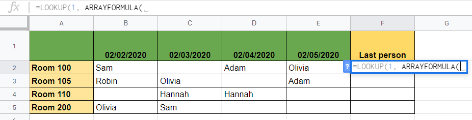
- After the opening bracket ‘(‘, you have to add the variables. Depending on which solution you use, you can add 2 or 3 variables. For this guide, I will go through the steps of Option #2, but you can do the same with the variables of Option #1 as well.
- Add the first variable, which is the key value we are looking for. We look up 1, so this is the first variable.

- After that, add the
search_rangevariable, which is theARRAYFORMULAconverting the cells into numbers. Start writingARRAYFORMULAand add the bracket to start writing its content.
- Now we write the cell range where we want to perform the
LOOKUPfunction. It is B2:E2 when we work on row 2.

- To check whether those cells in the row are empty or not, we include the not-equal expression that returns TRUE when the cell is not empty and FALSE when it is empty. This expression is B2:E2 <> “”.

- Now we divide 1 by this expression to convert the TRUE and FALSE values into a form that the
LOOKUPfunction can handle.

- After the second variable is done, add the third variable which is
result_range. It is the range of cells that you use for the lookup, so the range B2:E2.

- Finally, close the brackets and hit Enter. You can see the last name of row 2.
- At last, drag down this function to the rest of the rows to apply it to the other rooms.
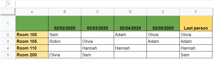
That’s it, good job! You can now use the LOOKUP function to find the last value in each row in Google Sheets. Feel free to use it together with the other numerous Google Sheets formulas to create even more powerful formulas that can make your life much easier. 🙂


1 comment
well explained. I have a question. What if I want to get the last number if this range has both strings and numbers? What kind of changes do I need to do?