How to Match Multiple Values in a Column in Google Sheets

Knowing how to match multiple values in a column in Google Sheets is useful if you need to check if multiple values are available within an array in your spreadsheet.

Let’s take a look at one example, to make it easier for everyone to understand!

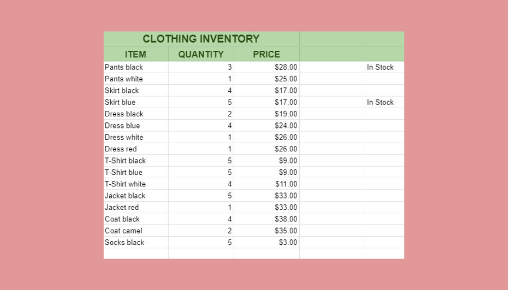
Say you own a clothing store and someone wants to order three garments (black pants, blue dress, and white t-shirt) but wants them only if all three of them are in stock. 

How should we go about this problem?

We will create our own formula that will look through our clothing inventory to see if all three required garments are available and return ‘In Stock’ if they are, or ‘Out of Stock’ if they are not.

There are two ways we can do this, and we will explain both of them. Let’s now take a closer look at our two formulas and how each of them works in a spreadsheet!

How to Match Multiple Values in a Column in Google Sheets (Using the REGEXMATCH Function)

The first formula we will use to match multiple values in Google Sheets is =IF(SUM(ArrayFormula(IF(LEN(A3:A),ArrayFormula(–REGEXMATCH(A3:A, “Pants black|Dress blue|Coat black”)),””)))>=3,”In Stock”, “Out of Stock”).

As you can see, we used the REGEXMATCH,  IF, LEN, and  ArrayFormula functions to build it. We have already explained how IF, LEN, and ArrayFormula functions work butREGEXMATCH is new to us. In the following section, we will explain its anatomy.

The Anatomy of the REGEXMATCH Function

The syntax (the way we write) the REGEXMATCH function is especially simple, and it is as follows:

=REGEXMATCH(text, reg_exp)

Even though the syntax is simple, we will explain it for those who do not know what each of these terms means:

• = the equal sign is the sign you will find at the beginning of every function in Google Sheets.
• REGEXMATCH() is our function.
• text the string or value we are going to test to see whether it matches the regular_expression.
• reg_exp is the regular expression to which we will compare the text.

⚠️ A Few Notes About Using the REGEXMATCH Function in Google Sheets:

The REGEXMATCH function supports various metacharacters, including:

• ^ which represents the beginning of the string
• $ which represents the end of the string
• . which represents a single character
• | which represents the Or operator
• [] which holds a set of characters and represents any one of the characters inside it
• [^] which holds a set of characters and represents any one of the characters not listed inside it
• \ which is used to escape a special character

A Real Example of Using the REGEXMATCH Function to Match Multiple Values in a Column in Google Sheets

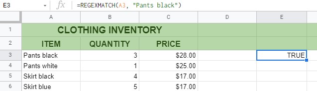
The simple formula with the REGEXMATCH function will be =REGEXMATCH(A3, “Pants black”). We will check if text from cell A3 matches the regular expression which is “Pants black”. Since the text matches the regular expression, our formula will return TRUE.

However, in our example, we need to match multiple values. This is why we will expand our formula. First, instead of just cell A3, we will be comparing the text from the whole column A, starting from the cell A3 (if we would want to compare the text from only several cells, we would insert the cell range, such as A3:A20). Then, we will use all three required garments as our regular expression but we will separate them with a metacharacter ‘|’ which represents an Or operation.

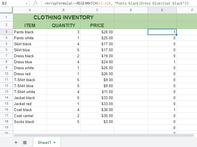
Now, since we are using the above formula in a column range, we will need the ArrayFormula. =ArrayFormula(–REGEXMATCH(A3:A20, “Pants black|Dress blue|Coat black”)). This will return ‘1’ where the text from the cell range A3:A20 matches one of the text strings from our regular expressions and ‘0’ where it does not.

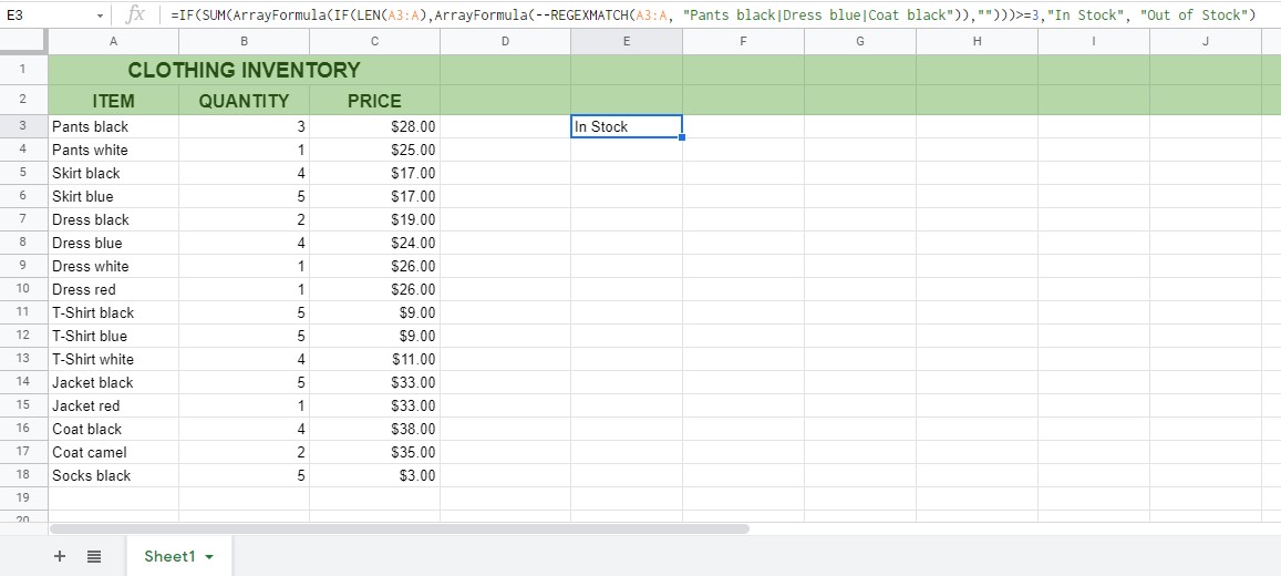
However, if you want to check an infinitive range (such as A3:A instead of A3:A20), you will need some help from the IF and LEN functions. The formula will now look like this =ArrayFormula(IF(LEN(A3:A),ArrayFormula(–REGEXMATCH(A3:A, “Pants black|Dress blue|Coat black”)),””)) and would return the results shown in the picture below:

Then, we will sum the above formula results. If the final result is equal to or greater than 3, we can be sure that all the three garments are available. To do this, we will use the formula shown at the beginning of this part of the article =IF(SUM(ArrayFormula(IF(LEN(A3:A),ArrayFormula(–REGEXMATCH(A3:A, “Pants black|Dress blue|Coat black”)),””)))>=3,”In Stock”, “Out of Stock”).

However, what you should know is that this formula will not work correctly if one of the values is missing and another one is repeating. Let’s say that there is no black coat on the list but there are two blue dresses. The formula will return ‘In Stock’ even though there’s no one of the garments we are looking for. This is when we can use another formula, we have built with the MATCH function instead.

How to Match Multiple Values in a Column in Google Sheets (Using the MATCH Function)

The other formula we can use to match multiple values in Google Sheets is =IFERROR(IF(AND(MATCH(“Pants black”,A3:A,0)+MATCH(“Dress blue”,A3:A,0)+MATCH(“Coat black”,A3:A,0))>0,”In Stock”),”Out of Stock”). 

We have created this formula with the help of the MATCH function and the IF, AND logical test.

The Anatomy of the MATCH Function

The way we write the MATCH function is as follows:

=MATCH(search_key, range, [search_type])

We will explain the syntax for those who do not know what each of these terms means:

• = the equal sign is how we start any function in Google Sheets.
• MATCH() is our function.
• search_key is the value we will search for within the range.
• range the one-dimensional array to be searched for the search_key.
• search_type is the manner in which to search [optional].

1 By default. It causes the MATCH function to assume that the range is sorted in ascending order and returns the largest value less than or equal to search_key.

0 Indicates exact match (you’ll need it if the range is not sorted).

-1 It causes the MATCH function to assume that the range is sorted in descending order and returns the smallest value greater than or equal to search_key.

You can find more about the MATCH function in our article ‘How To Use INDEX and MATCH Together in Google Sheets’.

A Real Example of Using the MATCH Function to Match Multiple Values in a Column in Google Sheets

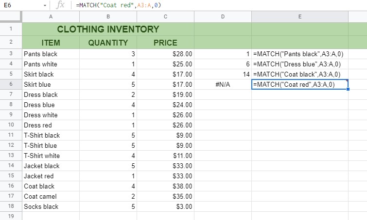
When we break down our formula, we will get =MATCH(“Pants black”,A3:A,0). This simple formula will return the relative position of an item within a selected range. In our example, that is 1. For the =MATCH(“Dress blue”,A3:A,0) formula, the result would be 6, and for =MATCH(“Coat black”,A3:A,0) it would be 14. If any of the items we were searching for is not available, the formula would return #N/A error.

Now, we would want to test if all of the above items are returning relative position numbers. We can do that with the help of IF, AND logical test. The formula we will use is =IF(AND(MATCH(“Pants black”,A3:A,0)+MATCH(“Dress blue”,A3:A,0)+MATCH(“Coat black”,A3:A,0))>0,”In Stock”). This means that if the value is greater than 0 (when all of the items are available in the list), the formula should return ‘In Stock’.

Finally, we will add the IFERROR function, to return ‘Out of Stock’ if any of the items is not available in the list and the #N/A error appears.    

That is it! Now you know how to match multiple values in a column in Google Sheets using two different formulas! And you have learned more about the REGEXMATCH and MATCH functions.

If you want to practice some more, make a copy of our spreadsheet and give it a try:

Or browse our other Google Sheets formulas and make even more powerful formulas you can use to sort, filter, match, and highlight your data. 🙂

Get emails from us about Google Sheets.

Our goal this year is to create lots of rich, bite-sized tutorials for Google Sheets users like you. If you liked this one, you'll love what we are working on! Readers receive ✨ early access ✨ to new content. There will be no spam and you can unsubscribe at any time.

Subscribe