The RANK.AVG function in Google Sheets is used to determine the rank of a specific value in a given dataset.
If there are two or more entries of the same value in the dataset, the average ranks of those entries shall be returned.
Table of Contents
The rules for using the RANK.AVG function in Google Sheets are as follows:
- The values placed in the
RANK.AVGfunction should be numeric values. - Values considered should be a part of the dataset specified.
- The function returns an integer corresponding to the specified value’s rank when sorted in ascending or descending order.
The RANK.AVG function is a statistical function that works similar to the RANK and RANK.EQ function. While all three functions determine the rank of a number and even have the same parameters, the RANK.AVG function distinguishes itself when entries with the same value are present. Instead of returning the top rank of those values, it returns the average of their ranks.
Consider this example.
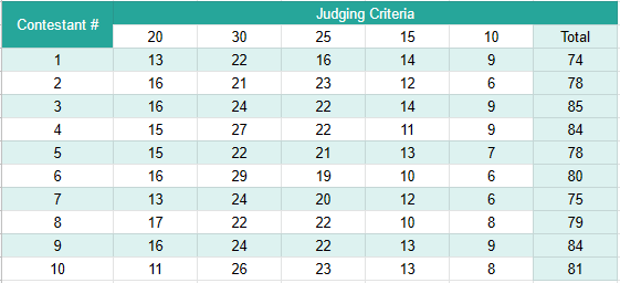
You were tasked to create a spreadsheet that will automatically calculate the total scores of each participant in a stage play competition. It should also determine the rankings without the need of rearranging the total scores from highest to lowest. From the given judging criteria, the point gained for each will be summed up to determine a participant’s score. The team with the highest score will be declared the winner.
To determine if your spreadsheet will work, you input sample scores and managed to create a spreadsheet that can calculate the participants’ total score. The example spreadsheet you drafted is shown below.

If there will only be a limited number of participants, determining the rankings can be done by taking a glance at the total scores. An increased number of participants, however, will make this significantly more difficult and prone to error. As such, you will need to find a way to automate this process to ensure that the rankings you determine will be accurate. When a tie occurs, you wish for their ranks to be presented as an average instead of the top rank of those scores. How can you do so?
The RANK.AVG function is the exact function for this situation. It returns the rank of a specific value in a given dataset and assigns the average rank of repeated values if they are present. Ranks may be based on ascending or descending order.
Let’s get to know more about the RANK.AVG function in Google Sheets!
The Anatomy of the RANK.AVG Function
So the syntax (the way we write) the RANK.AVG function is as follows:
=RANK.AVG(value, data, [is_ascending])
Let’s dissect this thing and understand what each of these terms means:
=the equal sign is just how we start any function in Google Sheets.RANK.AVG()this is ourRANK.AVGfunction. It returns the rank of a specific value in a dataset. When multiple entries have the same value, their ranks will be equal to the average rank of those entries.valueis the value whose rank will be determined. This value may be specified in the formula or it may be a cell reference.datais the array or range that contains the dataset from where the rank of value will be obtained from. Ifdatadoes not contain thevaluein any cell or element, theRANKfunction will return the #N/A error.is_ascendingdetermines how values indatawill be arranged. The square brackets ‘[]’ indicate that this is an optional parameter. By default, its value is FALSE when not specified – indicatingdatato be arranged in descending order. If a value of TRUE is used,datawill be arranged in ascending order. This means that the least value will have a rank of 1.
A Real Example of Using the RANK.AVG Function
Take a look at the example below to see how RANK.AVG functions are used in Google Sheets.

As you can see, the RANK.AVG function ranks the highest value in the dataset as 1 when the is_ascending parameter is not specified. If you want the lowest value to be ranked first, then this parameter should be specified as TRUE.
Entries that have the same values are highlighted in the example. Notice how the rank returned for these values is the mean of the rank placements. Looking at the data, the value of 15 is repeated twice, and such should occupy the 3rd and 4th positions in column B. Since these two entries are tied, the rank returned is presented as the average of these positions which is 3.5.
When an odd number of entries have the same value, the middle rank will be returned. Such as the case with the entries with the value of 2 that should occupy the last 3 ranks when arranged in descending order. All of the entries are ranked as 9.
You may make a copy of the spreadsheet using the link I have attached below:
How to Use the RANK.AVG Function in Google Sheets
Now, let’s finally use the RANK.AVG function to solve the example showed earlier.
- Simply click on any cell to make it the active cell. For this guide, I will be selecting H3 where I want to show my result.

- Next, simply type the equal sign ‘=’ to begin the function and then followed by the name of the function which is our ‘rank.avg’ (or ’RANK.AVG’, whichever works). You should find that as you are typing, an auto-suggest box appears with the names of the functions that contain the text that you have typed. The one we want is the RANK.AVG function, so make sure to click on the RANK.AVG function.

- Now, we need to specify what the
valueto be ranked should be. For this example, I will first determine the rank of contestant 1. Select cell G3 and insert a comma ‘,’ to indicate that we would now like to input thedataparameter.

- To specify the
dataparameter, select the array containing the dataset to be considered. These are the values in cells G3:G12. Simply select this range and convert it to an absolute cell reference by pressing F4 on your keyboard once. This allows you to copy the formula down while keeping the same set of values for the data parameter.

- Since we want the highest value to be ranked as the highest, let’s just leave the
is_ascendingparameter blank. Press Enter to finish the formula. To complete the table, simply copy the formula to the other rows.

To further improve this spreadsheet and be able to determine the rankings regardless of the number of entries in the dataset, let’s discuss how to use other functions alongside the RANK.AVG function. We shall make use of the ARRAYFORMULA and IFNA functions to easily determine the rank of values regardless of dataset size.
The ARRAYFORMULA function allows you to only edit the formula in one cell and the remaining cells will be automatically filled up. To learn more about this function, feel free to follow the link provided.
The IFNA function is a more specific version of the IFERROR function that allows you to specify a value when a formula returns the #N/A error. We already know that the RANK.AVG function returns the #N/A error when the value specified is not a part of the dataset considered. Therefore, any of the two functions can be used.
When you apply these two functions along with the RANK.AVG function for the example earlier, you should end up with the following table:

As you can see, you only need to input the formula for one cell and the remaining values will automatically be filled. Even though we have selected the entire G column as a part of the data set, an error prompt did not show because of the IFNA function.
Exploring conditional formatting options can also help in improving this spreadsheet. For this example, we can see that there are actually two sets of ties, a set tied for 2nd and 3rd place and another for 7th and 8th place. Setting up conditional formatting for duplicate ranks or highlighting the first 3 places are a few options to explore but will no longer be discussed in this article.
That’s pretty much it. You can now use RANK.AVG functions in Google Sheets together with the other numerous Google Sheets formulas to create even more powerful formulas that can make your life much easier.


