How to Use INDIRECT Function in Google Sheets

The INDIRECT function in Google Sheets is useful if you want to return a cell reference specified by a string.

The function is often used as a referencing tool in a formula to a cell or range that is readily available.

Let’s take an example:

By selecting A2, the return value would be “123”, as it is the cell reference in A4.

The INDIRECT function only understands cell reference addresses in Google Sheets. Hence, by selecting A3, the return value becomes “#REF!”, meaning the formula is not valid.

This is because the INDIRECT function could not understand “Hello” as it is just plain text and not a cell reference address that the function can refer to.

The INDIRECT function would be really handy in real-world situations!

 

 

The Anatomy of the INDIRECT Function

The way we write the INDIRECT Function is: 

=INDIRECT(cell_reference_as_string, [is_A1_notation])

Let us help you understand the context of the function:

• The equal sign =  is how we start any function in Google Sheets.
• INDIRECT() is our function. We need to add two attributes, namely the cell_reference_as_string and [is_A1_notation], to make it work correctly. 
• The cell_reference_as_string is a cell reference, written as a string.
• The  [is_A1_notation] is an expression used to indicate what style notation to display the cell reference in. This attribute is optional. 

Let’s have a more detailed understanding of what [is_A1_notation] means.

Is A1 Notation:

This attribute is to determine how the cell reference’s address would be displayed.

Here are the references:

 

 

A Real Life Example of Using INDIRECT Function

Example 1

Let’s use a real-life situation to utilize the INDIRECTfunction to show how powerful this function can be!

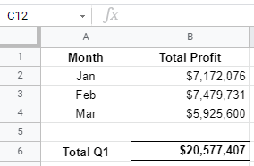
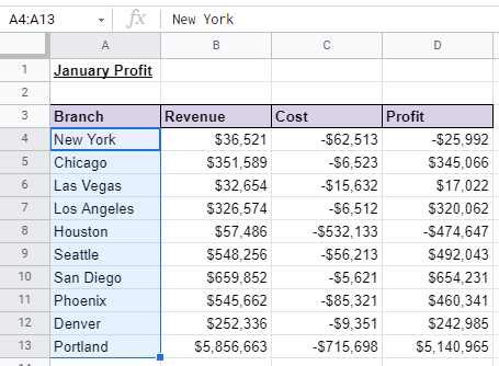
Here is a summary of the total profit for the first quarter of 2020 that is linked to different month’s tab. 

This example would show how to use the INDIRECT function to refer cell references from several other tabs. 

 

 

How to Use INDIRECT Function in Google Sheets

1. Simply click on the cell that you want to write down your function at. In this example, it will be B2.

 

2. Begin your function with an equal sign =, followed by the name of the function, SUM, and an open parenthesis(.

 

3. Add INDIRECT, then another open parenthesis(.

 

4. We will select A2 as our cell_reference_as_string.

By selecting A2, we are referring the formula to the tab named ‘Jan‘.

 

5. Then, add an ampersand& to join two or more text strings in a single string.

 

6. Next, enclosed by a quote-unquote symbol "", select the cell we want to refer to.

We have selected “!B4:D13” as this is the range of cells where the profit would be sum-up in all three tabs.

 

7. After the following steps, your input should look like this:

 

Example 2

Let us show you how to use the INDIRECT function in a more complex formula.

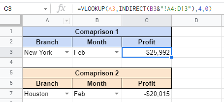
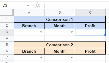
By using a mixture of functions and tools in Google Sheet, we have created a template to perform profit comparisons between different branches in different months. 

Here is a rundown of the tools and functions involved:

1. Data Validation tool – restricts the type of data or the values a user enters into a cell. In our case, it creates a drop-down to select which branch and month we would like to use as a comparison.  
2. VLOOKUP function – helps pull out data from a complex database or tables.

For more in-depth explanations and examples for the VLOOKUP function, click here!

 

1. To create data validation on a cell. First, select the cell you want to validate, which is A3.

 

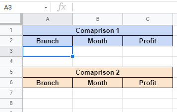
2. Next, click on ‘Data‘ on the Google Sheet Toolbar.

 

3. Select ‘Data Validation‘.

 

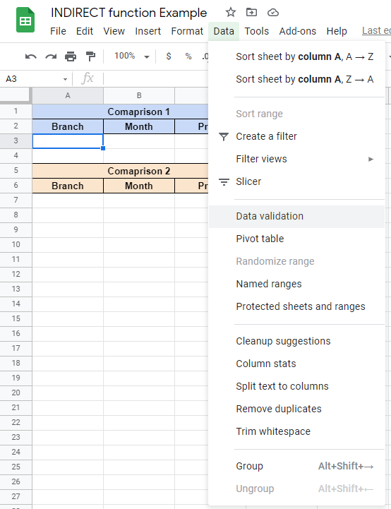
4. Once clicked, this is what would display on your screen:

 

5. Then, select the range of data you would like to validate. Using the same database as Example 1, we have selected all the branch names. Simply select the listed branch name from any tab.

 

6. After selecting the range of data, click Save.

 

7. After clicking Save, the cell would display an arrow that would drop down to a list of branch names.

 

8. Do the same for the “Month” column.

You can also manually list down the items.

 

9. Now let’s move on to the formula. VLOOKUP function has four attributes, search_key, range, index, and [is_sorted].   

 

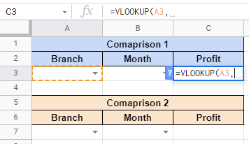
10. First, click on the cell you want to write the formula in. In this example, it would be C3.

 

11. Begin your function with an equal sign =, then followed by the name of the function, VLOOKUP, then an open parenthesis(.

 

12. Next, select the search_key that we would like to search, which is A3.

 

13. Then, we will add the INDIRECT function as the range we would like to search from.

 

14. Just like Example 1, we will enter the range we want to search from, which is the cell_reference_as_string attribute. 

 

15. Lastly, we will insert ‘4‘ as the index, meaning the column of the value to be returned. The last attribute is optional, but inserting 0 or False is recommended to get a more accurate return value.

 

16. The formula is now done! Simply select which branch and month you would like to compare and the profit would automatically show! ✨

You may make a copy of the spreadsheet using the link attached below and try it for yourself:

That’s about it! You can now use the INDIRECT function in Google Sheets together with the other numerous Google Sheets formulas to create even more powerful formulas that can make your life much easier.