How to Use MIN Function in Google Sheets

The MIN function in Google Sheets is useful when you need to return the minimum value in a numeric dataset.

The minimum value is the result of comparing numbers in a specific dataset and finding the number that all other numbers in the dataset are greater than or equal to.

The rules for using the MIN function in Google Sheets are as follows:

• The function requires at least one argument, which may be a value, cell, or cell range.
• The function then outputs the minimum value out of the arguments provided.

Let’s take a look at an example of where we can use the MIN function.

Let’s say you’re shopping for a new phone. You have a list of potential choices available, as well as discounts available on those platforms. Given the discounted prices, which phone is the cheapest option?

With the MIN function, we can easily find the choice that will cost us the least amount of money.

The MIN function is useful for cases where you need to find the smallest value in a list. Later, we’ll go through how we can use the data provided and the MIN function to return the result we need. For now, let’s look into how the MIN function works.

The Anatomy of the MIN Function

The syntax of the MIN function is as follows:

=MIN(value1, [value2, ...])

Let’s take apart this formula and understand what each of these terms means:

• = the equal sign is how we start any function in Google Sheets.
• MIN() is our MIN function. It returns the minimum value in a numeric dataset.
• value1 refers to the first value or range to consider when computing the minimum value.
• value2 refers to additional values or ranges to consider when finding the minimum value.
• Text values found in the arguments will cause it to return a #VALUE! error.

A Real Example of Using MIN Function

Let’s look at a real example of the MIN function being used in a Google Sheets spreadsheet.

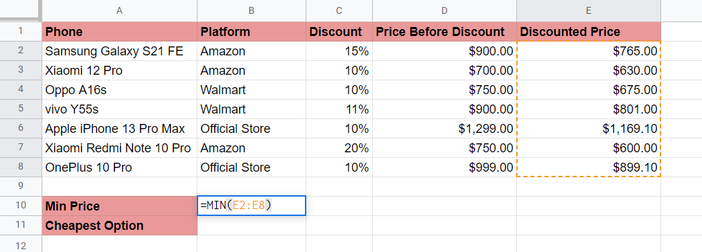
In the table below, we have our list of cell phone options along with their computed discount price. Using the MIN function, we were able to find out that the cheapest option is worth $600. 

To get the value seen in cell B10, we just need to use the following formula:

=MIN(E2:E8)

The MIN function only returns the value, so we manually checked which option corresponds to the minimum price. If you want to get this using a formula, we can use the INDEX and MATCH functions. 

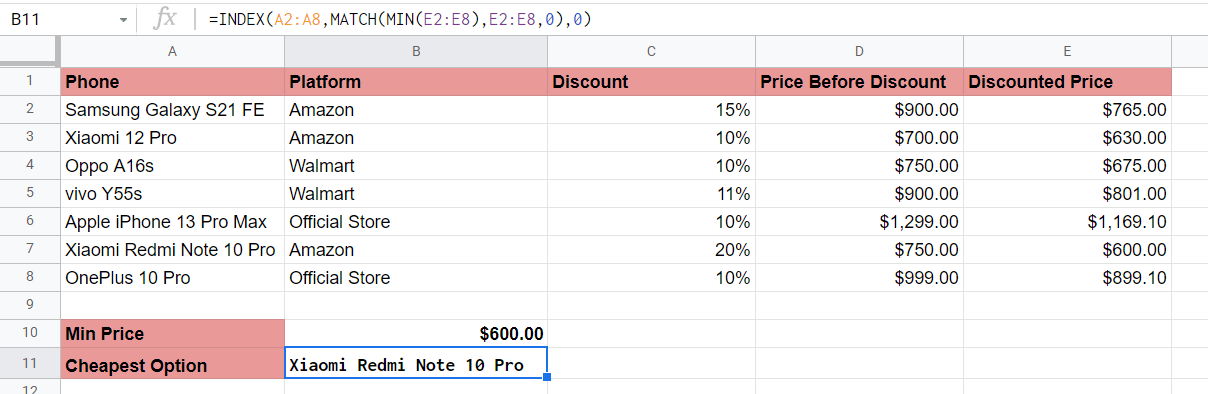
To get the cheapest option on our list, we can use the following formula:

=INDEX(A2:A8,MATCH(MIN(E2:E8),E2:E8,0),0)

Let’s quickly break this down. The INDEX function requires three arguments: a range, a row offset, and a column offset. Since we want INDEX to return the name of a phone, we’ll use A2:A8 as our range. The column offset remains 0 since we only need to look at one row for now. 

The MATCH function returns the relative position of an item in a range that matches a specified value. In this formula, we’re finding the cell that matches the smallest value in the E2:E8 range (which we find using the MIN formula). In this case, the MATCH function returns 6 since $600 can be found in the 6th place of the given range. An offset of 6 in range A2:A8 gives us the Xiaomi phone. 

You can make your own copy of the spreadsheet above using the link attached below. 

If you’re ready to try out the MIN function in Google Sheets, let’s begin writing it ourselves!

How to Use MIN Function in Google Sheets

In this section, we will go through each step needed to start using the MIN function in Google Sheets. This guide will show you how to find the cheapest item in a list, as seen in the previous examples.

Follow these steps to start using the MIN function:

1. First, select the cell which will hold the result of our MIN function.
   
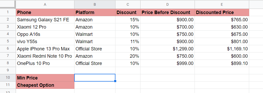
2. Next, we just have to type the equal sign ‘=‘ to begin the function, followed by ‘MIN(‘.  
3. You may find a tooltip box with tips on how to use the current function. Click on the arrow found in the top-right-hand corner of the box to hide it from view.
   
4. Next, we’ll select the range of values to find the minimum value. In this case, we’ll be looking for the minimum value in the range E2:E8.
   
   
   Afterward, we can simply hit Enter to let the function evaluate. We can also get the name of the phone using the INDEX and MATCH formula mentioned in the previous section.
   

Frequently Asked Questions (FAQ)

1. When should I use the MIN and MINA functions?
   The main difference is that the MINA evaluates TRUE and FALSE values as 1 and 0, respectively. The MIN function only considers numeric values when finding the result. If your dataset contains logical values, then it is suggested to use the MINA function instead.
2. Will non-numeric values return an error?
   The MIN function will just ignore all non-numeric values in the provided dataset. If no numeric values are found in the arguments, the MIN function will simply return 0.

That’s all you need to remember to start using the MIN function in Google Sheets. This guide shows how simple it is to use the MIN function to find the largest value in a dataset.  

The MIN function is just one example of a mathematical function in Google Sheets. With so many other Google Sheets functions out there, you can surely find one that best suits your worksheet.

Make sure to subscribe to our newsletter to be the first to know about the latest Google Sheets guides and tutorials from us. 

Get emails from us about Google Sheets.

Our goal this year is to create lots of rich, bite-sized tutorials for Google Sheets users like you. If you liked this one, you'd love what we are working on! Readers receive ✨ early access ✨ to new content.

Subscribe