


The RRI Function in Google Sheets is useful if you want to calculate the interest rate of a given investment with specified present value, future value, and time.
Table of Contents
The RRI function does this simply by identifying the number of periods the investment is made, its present value, and the future value. The present and future values are expressed in dollar amounts (or other currencies for that matter).
Let’s take an example to understand the concept better.
Say I had invested my salary bonus of $10,000 to an investment that would yield to $20,000 in 5 years. I want to check the interest needed in order for my investment to grow to $20,000 in 5 years.
How do we do that?
It’s easy. We can use the RRI function to check the rate of return just by supplying all the given – the period, present value, and future value. Ultimately, the RRI function will yield to a decimal number. But, you could easily transform it to a percentage value either by using the percent function (%) or by editing it in the Format tab in Google Sheets.
That’s how the RRI function works.
This function is handy especially when you are trying to test out which investment has the highest or lowest interest rate. This is also essential when you are trying to see if the investment is worth investing for, or otherwise.
In the world of investments, an algebraic formula is used to solve for the interest rate. But, it is made simpler with the help of Google Sheets.
Just imagine, you are given 3 different investment options, each will grow to $150,000, but the periods are not the same. Say 3 years for Investment A, 2 years for Investment B, and 1 year for Investment C. Instead of computing these manually, using the RRI function, you can simply supply the attributes needed and you can instantly see the interest rate for each of the investments. From there, you can now decide which among the investments is the best.
Let’s now dive into a real scenario where we will give you actual values and how we can write our own RRI function in Google Sheets to compute those data.
The Anatomy of the RRI Function
So, the way we write the RRI function is:
=RRI(number_of_periods, present_value, future_value)
Let’s break this down to understand better what each attribute means:
=the equal sign denotes the start of our function, like how we start any function in Google Sheets.RRIis our function. To make this work, we need to add the other attributesnumber_of_periods,present_value,future_value, for it to work.number_of_periodsthe total number of years investment is made.present_valueis the current value of the initial investment.future_valueis the expected investment return after n years.
⚠️ Now a few notes when writing your own RRI function.
- All attributes except the
number_of_periodsshould always remain to be a positive value. - An error would occur if the
present_valueis 0. - Make sure the
number_of_periodsis not blank nor equal to 0 to avoid a #DIV/0! error.
The Two Ways to Express the Final Answer
There are two easy ways to express our answer, and we will show you all those and their corresponding steps.
-
In 2 Decimal Places
If you opt to express the final answer in just 2 decimal places, you can simply select the answer, then click the Format tab in Google Sheets. Click on ‘Number‘. It will show a drop-down menu on the side. Scroll down to ‘More formats‘, then choose ‘Custom number formats‘. After this, select the first option (0.00), and it will magically convert the answer into 2 decimal places.
Another way to show this, and probably faster, Look for the ‘Decrease decimal places‘ tab found beside the percent sign (%) in Google Sheets. Click on that button until you reach the 2 decimal places.
-
Percent Value
Another way is to express it in percent value – which is very common. To do this, click the Format tab, then click on Number. Look for the word ‘Percent‘, then click it.
Additionally, perhaps the easiest way to convert a decimal value to a percentage value is to simply find the percent icon (%) in Google Sheets and click it. Your RRI answer will automatically transform to a percent value.
It may seem confusing up to this point, but we assure you that after reading this guide, you will surely feel comfortable applying the RRI function in Google Sheets. So hang in there! 🙂
A Real Example of Using RRI Function
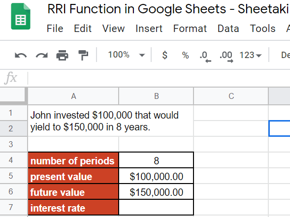
Take a look at the example below to see how RRI function is used in Google Sheets.

As you can see in the example above, we used the RRI function to determine the needed interest rate for John’s investment to grow from $100,000 to $150,000 in 8 years.
The formula is:
=RRI(B4,B5,B6)
Here’s what this example does:
- We carefully identified the given information – the number of years, present value, and future value, and wrote them down beside their respective labels.
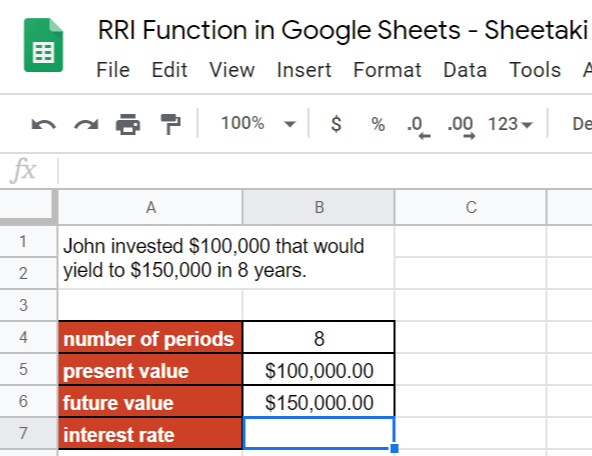
- Next, we selected cell B7. This is where we will write our working
RRIformula. - We started off by selecting B4 which is the number of periods, or the number of years. In this case, it’s 8 years.
- Then, we clicked on B5, which represents the present value of the investment. For this guide, our B5 is worth $100,000.
- Ultimately, we clicked on B6, our future value. This is the expected return of our investment after the 8th year. For this guide, B6 is equivalent to $150,000.
- The moment we closed our formula and hit on the Enter key, it resulted in a decimal value of 0.05198950551.
- Since we wanted to have this as a percentage value, we will then click the cell B7 where the answer is, and click the percent sign (%) just beside the dollar sign ($) in Google Sheets.
- There you have it! The decimal point is automatically changed to a percentage value.
That’s how easy it is.
You may make a copy of the spreadsheet using the link I have attached below:
Feel free to make a copy of the example spreadsheet for the RRI function which we discussed above to try and see how it is done. Experiment with it and you will go through the above steps once again on your own using different sets of data.
Now let’s begin writing our own RRI function in Google Sheets.
How to Use RRI Function in Google Sheets
- The first step is to identify our function’s attributes. In the given scenario, we conclude that the number of years is 8, the present value of John’s investment is $100,000, and the yield or the future value is $150,000.
- After identifying all the given, we will then make any cell active. This is where we want to write our formula. In this guide, I selected B7.
- Next is to start our formula with an equal sign followed by the
RRIfunction. Add an open parenthesis “(” so that at this point, you will see a pop-up message that will serve as your guide in writing our formula.
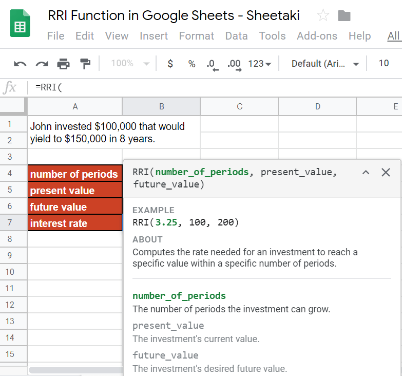
- Since we’ve already identified our needed data, all we have to do is to select the cells that contain the period, present value, and future value. For this guide, we will then click B4, B5, and B6.
- Hit on the Enter key.

- Since we want to express our answer in a percentage form, we will click on the percent sign (%) found beside the dollar ($) sign in Google Sheets. If you want to convert it back to decimal, then simply refer to the steps shared above under “The Anatomy of the RRI Function” section.
- At this point, you should see the final answer in a percentage form.

The final formula should look like this:
![]()
That’s pretty much it. You can now use the RRI function together with the other numerous Google Sheets formulas to create even more powerful formulas that can make your life much easier. 🙂


