How to Use COLUMN Function in Google Sheets

The COLUMN function in Google Sheets is useful to get the column number of a specific cell.

As the name of the function suggests, we can use this functionality to return the column number. We can return it of the same cell where we use this formula. We can even get the column number of any other referred cell in the sheet.

Let’s take an example.

Say we want to create a sheet and you need a numbering in the first row of your sheet. We want to have 1 in column A, 2 in column B and so on.

We don’t want to enter the column numbers one by one, but we want to do it in a more automated way.

So how do we do that?

Simple. The COLUMN function only needs the cell reference to output the column number.

Or even without a reference, we can output the column number of the same cell where we use this formula.

Let’s dive into some examples to show you how we can write our own COLUMN function in Google Sheets to calculate those data.

 

 

The Anatomy of the COLUMN Function

The syntax (the way we write) the COLUMN function is as follows:

=COLUMN([cell_reference])

Let’s break this down and understand what each of these terminology means:

• = the equal sign is how we start every function in Google Sheets.
• COLUMN is our function. We will have to add the values into it for it to work.
• cell_reference is an optional attribute which we can use in our function. It is the reference to the cell whose column number we require. If you don’t specify this attribute, the COLUMN function returns the column number of the cell where we enter the formula.

---

Return the Column Number of a Referred Cell

Have a look at the way the COLUMN function works.

Let’s write the following function in any cell:

=COLUMN(D2)

 

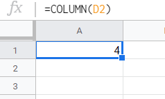
It’s pretty straightforward. It returns 4 because column D is the fourth column.

It doesn’t matter in which cell you use this formula as it still returns the column number of the cell D2.

---

Return the Column Number without Referring a Cell

As you can see, the single cell_reference attribute of this function is optional. So we can use this function without any attributes.

Let’s try it.

We put the following simple formula into every cell from A1 to E5:

=COLUMN()

 

The COLUMN function returns the column number of the cell that contains the formula.

As a result, we got the column numbers of these cells, where column A means 1, column B means 2 and so on.

---

Return the Column Number with a Referred Range of Cell

There is another thing we need to mention when discussing the syntax of the COLUMN function.

It is possible to add a reference to a range of cells instead of a single cell.

The function we write in cell A1 is as follows:

=COLUMN(C7:E12)

 

Now you might wonder what happens here.

Simple. The COLUMN function returns only the column number of the first column within the cell_reference and ignores the rest of the range.

Below we will be showing another example when we actually return the column numbers in a whole range of cells. But in that case, we will use an extra function too. Without any further functions, the COLUMN function only returns the column number of the first cell of the range.

 

 

A Real Example of Using COLUMN Function

Have a look at the example below to see how the COLUMN function is used in Google Sheets to output several column numbers.

 

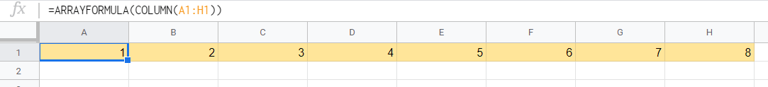
The example above shows how we used the COLUMN function to automatically fill out the column numbers. We did this without having to enter them manually.

Here we wrapped the COLUMN function into an ARRAYFORMULA function. The ARRAYFORMULA function is useful to apply a formula to an entire row or column in Google Sheets. Read more about its use in our previous article.

The function to fill out the column numbers is:

=ARRAYFORMULA(COLUMN(A1:H1))

Here’s what this example does:

• Firstly, we made a cell active. This is where we will start our ARRAYFORMULA and COLUMN formula. For this guide, we selected cell A1.
• Next, we started off our formula with an equal sign, followed by our first function, ARRAYFORMULA.
• After that, we wrapped the COLUMN function into it as its attribute.
• Then, we added the attributes of the COLUMN function, which is the range of cells where we wanted to return the column numbers. This is A1:H1 in this example.
• As a result, you can see the right column numbers from 1 to 8 throughout the cells A1 to H1.
• Note that here the ARRAYFORMULA takes care of applying the COLUMN function to all of the cells one by one that is referenced in the range. Unlike above in the section “Return the Column Number with a Referred Range of Cell”, the ranges are not ignored here. This is because of the way the ARRAYFORMULA function works.

See how simple that is!

Go ahead and give it a shot! 😀 Using the link I have attached below you can make a copy of the spreadsheet:

---

Modifying the Sheet After Using the COLUMN Function

Now let’s see how this solution exactly works. What happens to the numbering if we try to modify the columns?

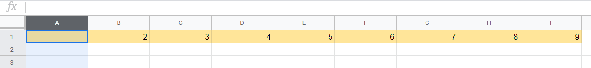
• Firstly, say we want to add a new column before column D.

 

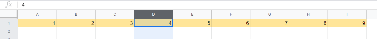
As you can see, we can add a column anywhere in between. The formula automatically readjusts the numbering, since it always returns the actual column number of the cells. With the additional column, our numbering changes to 1 to 9 now and expands until cell I1.

 

• Now let’s try adding a new column at the beginning, so before the current column A.

 

In this case, the new column is added, but it doesn’t have a numbering.

There is a simple reason for this.

When we added the new column, our ARRAYFORMULA wrapped COLUMN function didn’t move from its cell. Although it is now not called cell A1 but B1.

The function changed automatically according to the new column positions, so it is now as follows:

=ARRAYFORMULA(COLUMN(B1:I1))

Of course, it doesn’t mean that the function works wrong. It still outputs the column number of each cell as it is expected from cell B1 to I1.

 

 

How to Use COLUMN Function in Google Sheets

Let’s see how to write your own COLUMN function in Google Sheets step-by-step.

1. To start off, click on the cell where you want to start showing your results. For the purposes of this guide, I will be choosing A1, where I will write my formula.

 

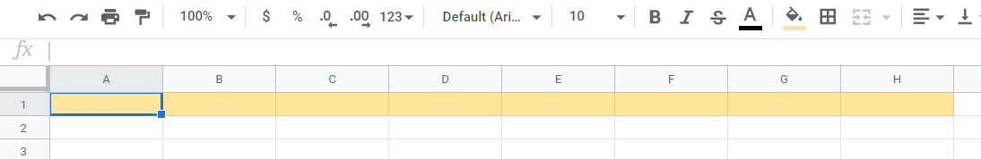
2. Next, type the equal sign ‘=’ to begin the function. Then followed by the name of the first wrapping function. It is the ‘arrayformula‘ (or ARRAYFORMULA, whichever works).

 

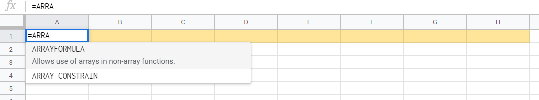
3. You should now see that the auto-suggest box will pop-up with the name of the function. Click on it to start your function.

 

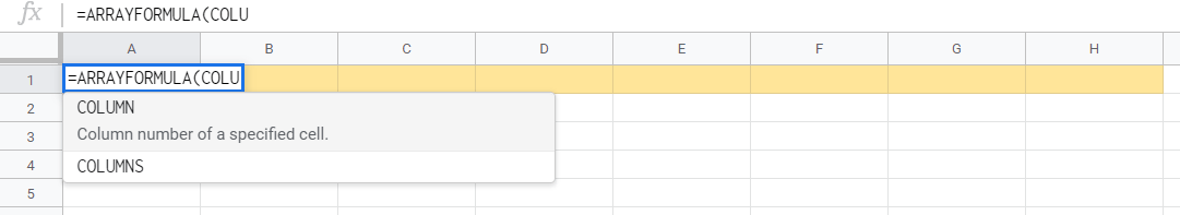
4. After the opening bracket ‘(‘, you have to add the COLUMN function. Start writing its name and again, select it from the pop-up auto-suggest box. Make sure to select the COLUMN function and not COLUMNS , which is a totally different function!

 

5. After that, add the range of cells whose column numbers you want to output. For example, I’m putting the range A1:H1 to return the column numbers of these cells. You can type the cell references manually, or you can simply click on them or highlight them to add them to your function.

 

6. Finally, if you added all the cells you wanted to include, hit the Enter key to close the brackets and get the result. Great! If you followed my steps, you would see the column numbers from A1 to H1.

 

That’s it, good job! You can now use the COLUMN function together with the other numerous Google Sheets formulas to create even more powerful formulas that can make your life much easier. 🙂