Converting seconds into a displayable HH:MM:SS format in Google Sheets can be hard, but once you learn how to do it, you’ll be able to make a functional time display with the HH:MM:SS format.
Table of Contents
In this article, we hope to teach you how to display HH:MM:SS using seconds. At the same time, we also aim to educate you on how you can use this by understanding the process behind this formula.
Google Sheets offer a variety of useful tools. Simple functions make our lives go round, but sometimes we come across a problem that requires a manual formula.
First off, why are we using seconds as raw data? The numbers are so large and inconvenient. Well, here’s why. Seconds are the building blocks of time.
To get minutes, you can divide a given number of seconds by the number of seconds in a minute (60 seconds). Following this line of thinking, we can also use seconds to get the day (86400 seconds) and the hour (3600 seconds). Once you get the right formula, you’ll be able to extract the days, hours, minutes, and seconds in a day and display it in HH:MM:SS format.
So how do we go about this?
Simple, we’ll use three functions to make this happen. A combination of the TRUNC, MOD, and TEXT function will help use display time in the HH:MM:SS format.
The Anatomy of the TRUNC Function.
The syntax (the way we write) of TRUNC functions is pretty simple.
=TRUNC(x,y)
Let’s breakdown what the function does and what the variables mean:
- = all functions begin with an equal sign in Google Sheets.
- TRUNC is a function that truncates a number. It might sound complicated, but it essentially just means cutting out all decimals unless specified not to.
- X is the number you want to be displayed.
- Y is the number of decimals you want to be displayed.
If you have X as 36.8888 and then have the Y value be 0. The number displayed will only be 36. You can also leave Y as blank to represent 0.
The Anatomy of The MOD Function.
=MOD(a,b)
The MOD function has a similar syntax, accepting only two variables. Here’s what these variables mean:
- = all functions begin with an equal sign in Google Sheets.
- MOD is a function that performs the modulo operator (%) on your number. This is programming jargon, it basically returns the remainder.
- A is the number you want to divide. The dividend.
- B is the number you’ll divide with. The divisor.
If you have A as 50 and then give B a value of 45. The number displayed will be 5 since that is the remainder of 50 / 45.
The Anatomy of The TEXT Function.
=TEXT(j,k)
The TEXT function also only accepts two variables. Here’s what these mean:
- = all functions begin with an equal sign in Google Sheets.
- TEXT displays a number into text according to a specific format.
- J is the number to be converted.
- K is the format you’ll use. For this tutorial, we’ll be using “MM:SS”. You can refer to the official list of formats here.
If you have J as 50 and then give K a value of “$0.00”. The number displayed will be $50.00.
A Real Example of Converting Seconds to HH:MM:SS Format
Let’s look at this example below to see how we can apply these functions in Google Sheets.
Displaying the HH:MM:SS Format of 60,000 Seconds in Google Sheets
In this simple problem, we’ll display 60,000 seconds in the HH:MM:SS format with the functions mentioned above.

The function with a cell reference is:
=trunc(C5/3600)&text(mod(C5/86400,1),":MM:SS")
Here’s how this works.
- TRUNC is responsible for finding the number of hours. It will divide A1 with 3600 and truncate/cut off any decimals. This will give us a clean number of hours.
- & is how you combine functions or text together.
- TEXT will automatically format the MOD function into minutes and seconds (MM:SS).
- MOD is in charge of separating minutes from days by dividing the given number of seconds by the seconds in a day (86400).
This simple problem can be practiced. Use the link below to use our spreadsheet sample:
How To Convert Seconds to HH:MM:SS Format in Google Sheets: Step-by-Step
- Let’s start by populating our sheets with the necessary data. For this guide, click on C3 and input the given number of seconds. We’ll use 69421 seconds for this tutorial.

- Now, click on D3 and type in ‘=’ to start off the function. Complete the function by typing in ‘trunc‘ or ‘TRUNC’. You will get auto-complete suggestions as you type. Feel free to auto-complete the function or continue typing.

- Next, let’s start entering the parameters by typing in ‘(‘ and input cell reference for the given numbers. In this example, it is cell C3.

- Finish the TRUNC function by adding ‘/3600)’. This will divide cell C3 with 3600, the number of seconds in an hour.

- Now we can proceed to the next half of the formula. Type in ‘&’ so we can begin adding these functions.

- Type in ‘text’ or ‘TEXT’ to call the TEXT function.

- We will be calling the MOD function inside the TEXT function. Go ahead and type ‘(mod’.
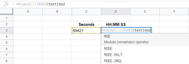
- On the same cell, add ‘(C3’ where C3 is the given number of seconds.
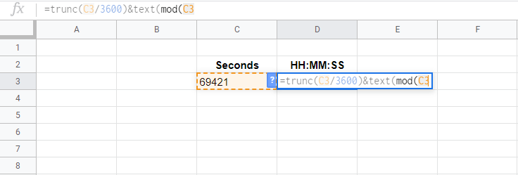
- Complete the parameter by typing in ‘/86400,1)’ which represents the number of seconds in a day and ‘1’ is the divisor.

- Continue by finishing the cell with “,“:MM:SS”)”. Don’t forget the comma, that’ll separate your function parameters. Adding this will tell the TEXT function how you want your data to be displayed. This will display your minutes and seconds.
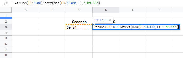
- Finally, the given number of 69421 should transform into the HH:MM:SS Format.
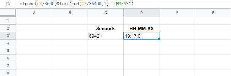
That should be all you need! Now you’ll be able to display seconds into HH:MM:SS. The TRUNC function was added so that you can have more than 24 hours displayed. If you want to display the number of days and hours, you can use this formula.
=trunc(x/86400)&" Day(s) "&text(mod(x/86400,1),"HH:MM:SS")
Are you the type to get into technical details? Here’s some trivia for you. If you notice and perform the MOD function yourself (mod(x/86400,1), you’ll most likely end up with a small number with an incredibly long line of decimals.
These decimals are then translated by the TEXT function and displayed into “HH:MM:SS”. This involves a lot of reverse-engineering that’s being done in the background. You can thank ingenious programmers for this!
And there you have it – you can now convert seconds to HH:MM:SS format in Google Sheets and use it together with the other numerous Google Sheets formulas to create even more effective formulas.