How to Use the DAY Function in Google Sheets

The DAY function in Google Sheets is useful to return the day of the month that a specific date falls on, in numeric format.

The DAY function is a simple and straightforward date function that can come handy if you are working with dates but only care about the days and want to get rid of everything else. You can also use it with some other formulas.

Let’s take an example.

Say you have a list of dates and want to know if a day from each date falls in the first half or second half of the month 📅

So how do we do that?

Simple. The DAY function just needs the date, and it will automatically return the day of the month that a specific date falls on, in numeric format. And with the help of the IF function, we can find out in which half of the month each of the days falls in.

Let’s first take a look at the anatomy of the DAY function, to help you understand how to use it in Google Sheets.

The Anatomy of the DAY Function

The syntax (the way we write) the DAY function is quite simple, and it is as follows:

=DAY(date)

Let’s break this down to help you understand the syntax of the DAY function and what each of these terms means:

• = the equal sign is how we begin any function in Google Sheets.
• DAY() is our function.
• date is the unit of time from which to extract the day of the month.

⚠️ A few notes you should know when writing your own DAY function in Google Sheets:

• Just like the MONTH function, the DAY function cannot read all human-readable dates. As the input value, you will have to use either a reference to a cell containing a date, one of the date functions such as NOW, TODAY, DATE or DATEVALUE, or a date serial number returned by the N function (for example, the underlying numeric value for the date ‘1/3/2020’ is 43833).
• If the date entered is not recognized as a number but as a text, the DAY function will return the error (#VALUE!).

A Real Example of Using the DAY Function

Let’s first take a look at how the DAY function works with different date values.

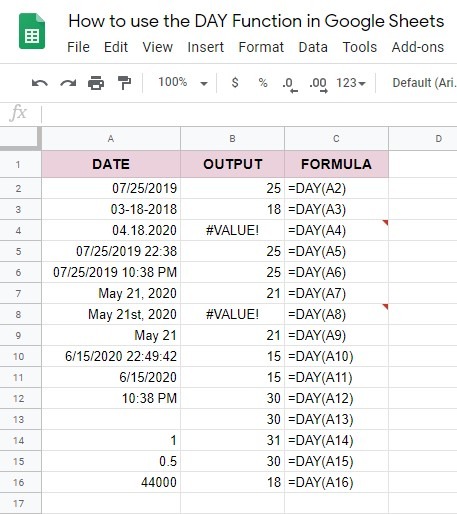
If you take a look at the first two dates (cells A2 and A3), you will see that these two are pretty simple. However, the input value in the third one (cell A4) is not recognized as a date and therefore the DAY function returned the error (#VALUE!).

Dates in cells A5 and A6 are the same as in the cell A2, just with the added time. As you can see, the DAY function is still able to return the day of the month that the date falls on.

If you take a look at the next three examples (cells A7, A8, and A9), you will see how the DAY function works when we use letters to write the name of the month. Two of them (cells A7 and A9) are recognized as dates, but the third one (cell A8) is not, and the DAY function returned the error (#VALUE!).

To write the dates in the cells A10 and A11, we used the NOW and TODAY functions. Both these inputs are recognized as dates by the DAY function. These two date values change, so the output will change as well.

The ‘zero’ date

If you take a look at the cell A12, you will see that there is no date, but the DAY function returned the day of the month that the date falls on. Now you must be wondering how is that possible. The solution is quite simple – when there is no date, the DAY function uses the ‘zero’ date (12/30/1899). The same goes if the cell is blank (cell A13).

When you input a random number into a cell (just like we did in the cell A14) and use theDAY function, the ‘zero’ date will be incremented by that value. This is why the output in the cell B14 is ’31’ (12/30/1899+1=12/31/1899). If you input only a decimal with no whole numbers, only the time will be incremented so the ‘zero’ date will stay the same.

To get near to the present date, you should enter 44000 (cell A16). The ‘zero’ date incremented by 44000 is 06/18/2020 so the DAY function will return ’18’.

You can make a copy of the spreadsheet using the link below and try it for yourself:

How to Use the DAY Function in Google Sheets

Let’s start writing our own DAY function in Google Sheets, so you can take a look at how it works and how to use it with other formulas.

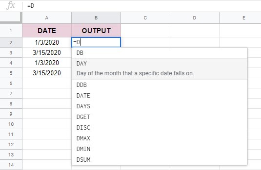
1. Click on a cell to make it active. For this guide, I will use the cell B2.

2. Type the equals sign ‘=’ and enter the name of the function, which is ‘DAY’. As you start typing, Google Sheets will auto-suggest the functions that start with the same letters. You can choose the DAY function from the list.

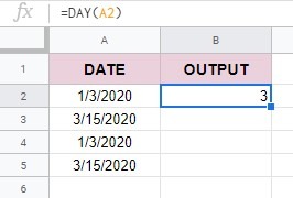
3. After the opening round bracket ‘(‘, input the date value. Since our date is already in column A, we will use the cell reference instead of typing the date into the DAY formula. Enter the A2 and close the function with a closing round bracket ‘)’. You can also press the Enter key on your keyboard, and the function will close automatically.

4. If you did everything right, the DAY function would return ‘3’. Now repeat these steps for the next row.

How to Use the DAY Function in Other Formulas In Google Sheets

Do you remember our example from the beginning of the text? How will you know if a specific date falls in the first half of the second half of the month?

For this, we will use the IF function.

Enter the formula as follows: =IF(DAY(A4)<15,”First Half”,”Second Half”) in cell C4 and =IF(DAY(A5)<15,”First Half”,”Second Half”) in cell C5.

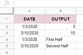
After adding the formula you should get the respective outputs that are evaluated based on the date that you have provided.

You can learn more on how to use the IF function in Google Sheets or take a look at the other Google Sheets formulas and learn how to create even more effective formulas that will help you with your data 🙂

Get emails from us about Google Sheets.

Our goal this year is to create lots of rich, bite-sized tutorials for Google Sheets users like you. If you liked this one, you'll love what we are working on! Readers receive ✨ early access ✨ to new content. There will be no spam and you can unsubscribe at any time.

Subscribe