

Calculating the Simple Moving Average in your Google Sheets document is useful as it makes your spreadsheet dynamic and flexible over time. It becomes increasingly easy to get lost in the rows and columns of data if you’re not careful with hard coding formulas and ranges. That’s why in the case of the Simple Moving Average, it’s best to use a changing formula while you use your spreadsheet. In this article, we will show you how to calculate the simple moving average in Google Sheets.
Table of Contents
What is the Simple Moving Average? It is one of the indicators used in technical analysis of trading and investing. It is called a “moving” average because you track the change of the value over time, usually a given number of days in finance. People often turn to it as it is simple to understand and even easier to construct.
For example, you are handling a chart focused on a certain stock and are keeping track of the changes every week, or every 7 days. After a while, the data list gets so long and the numbers can be so similar – it’s easy to lose track!
So, how should we proceed?
To accomplish our goal, we will use a combination of the GOOGLEFINANCE and the AVERAGE function of Google Sheets.
The Anatomy of the GOOGLEFINANCE and AVERAGE Function in Google Sheets
To get data on stock prices, we can use the GOOGLEFINANCE function. The syntax (the way we write) the GOOGLEFINANCE function is as follows:
=GOOGLEFINANCE(ticker,[attribute],[start_date],[end_date|num_days],[interval]))
Let’s break the function down to understand each term:
=the equal sign is how we begin any function in Google Sheets.GOOGLEFINANCEis our function. This is what we will use to fetch current or historical data from Google Finance.tickeris the ticker symbol for the company you want to analyze. Note that you need to specify which exchange symbol if you want to avoid some changes. In this example, “NASDAQ:GOOG” and “GOOG” both work.attributeis the attribute you want to retrieve from the Google Finance information. If left blank, it automatically retrieves price.start_dateis the first date when you want to get the historical data.end_date|num_daysis the end date when you want to get the historical data. Alternatively, you can add the number of days after thestart_date.intervalis the frequency of the data. This is either “DAILY” or “WEEKLY.”
The syntax of the AVERAGE function is simple:
=AVERAGE(value1,[value2,...])
=the equal sign is how we begin any function in Google Sheets.AVERAGEis our function.value1is the first value or range you want the function to consider.
We will combine these functions together to calculate the Simple Moving Average in Google Sheets.
A Real Example of Calculating the Moving Average
Let’s look at this example below to see how to use calculate moving averages in Google Sheets.
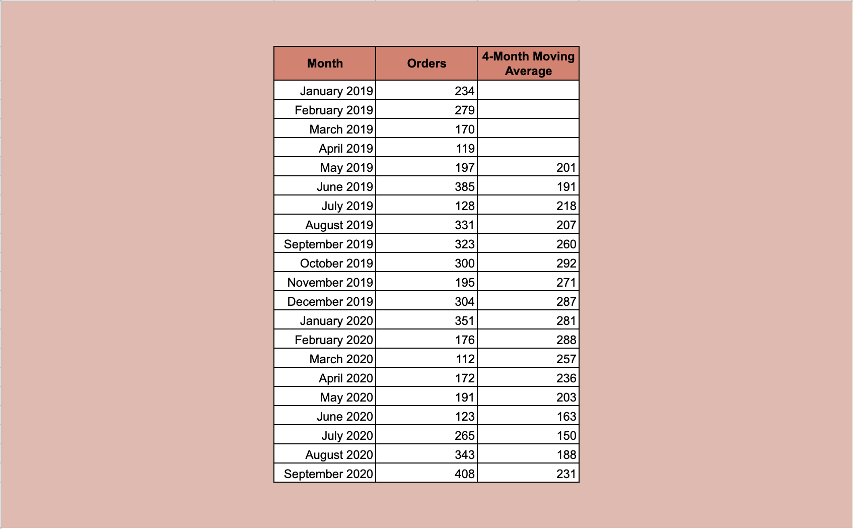
In this simple example, you want to find the 4-month moving average of the orders your business has received. You want to see the trend since you started in January 2019.
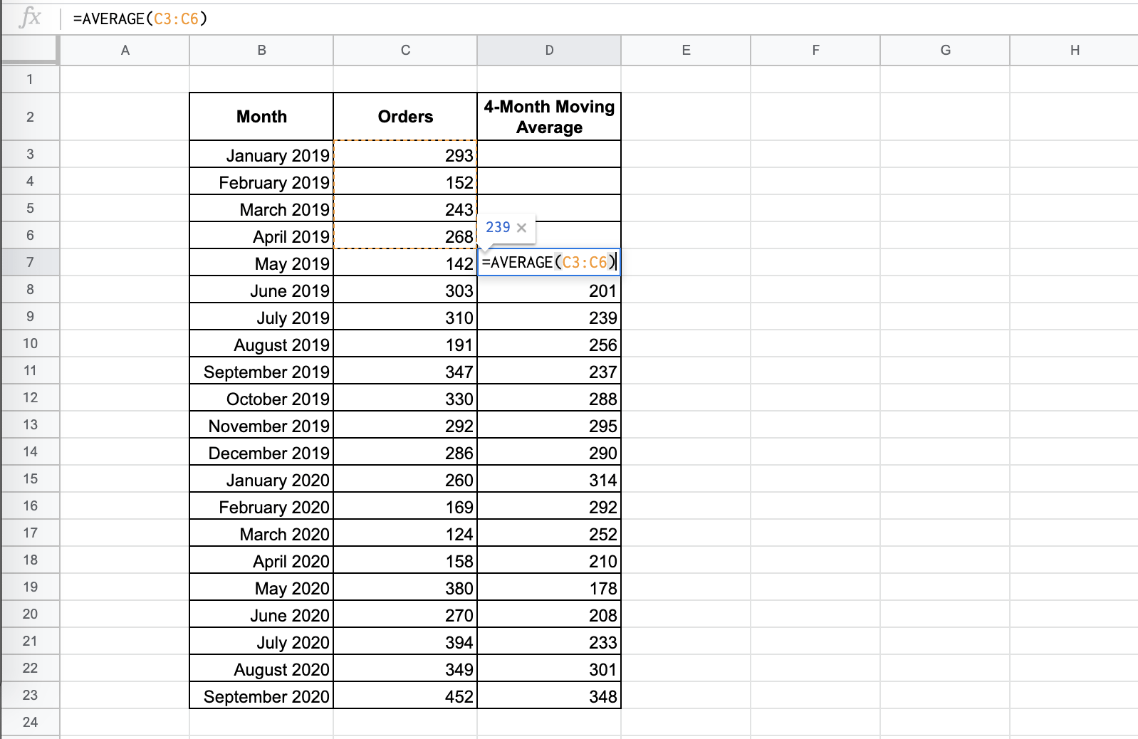
The column with the cell reference is:
=AVERAGE(C3:C6)
This formula has been copy-pasted down the column in order to calculate the average of the past 4-month’s performance.
This simple problem can be practiced. Use the link below to use our spreadsheet sample:
How to Calculate the Simple Moving Average in Google Sheets
Since Simple Moving Average is a finance tool, our example will feature the combination of the GOOGLEFINANCE and the AVERAGE functions.
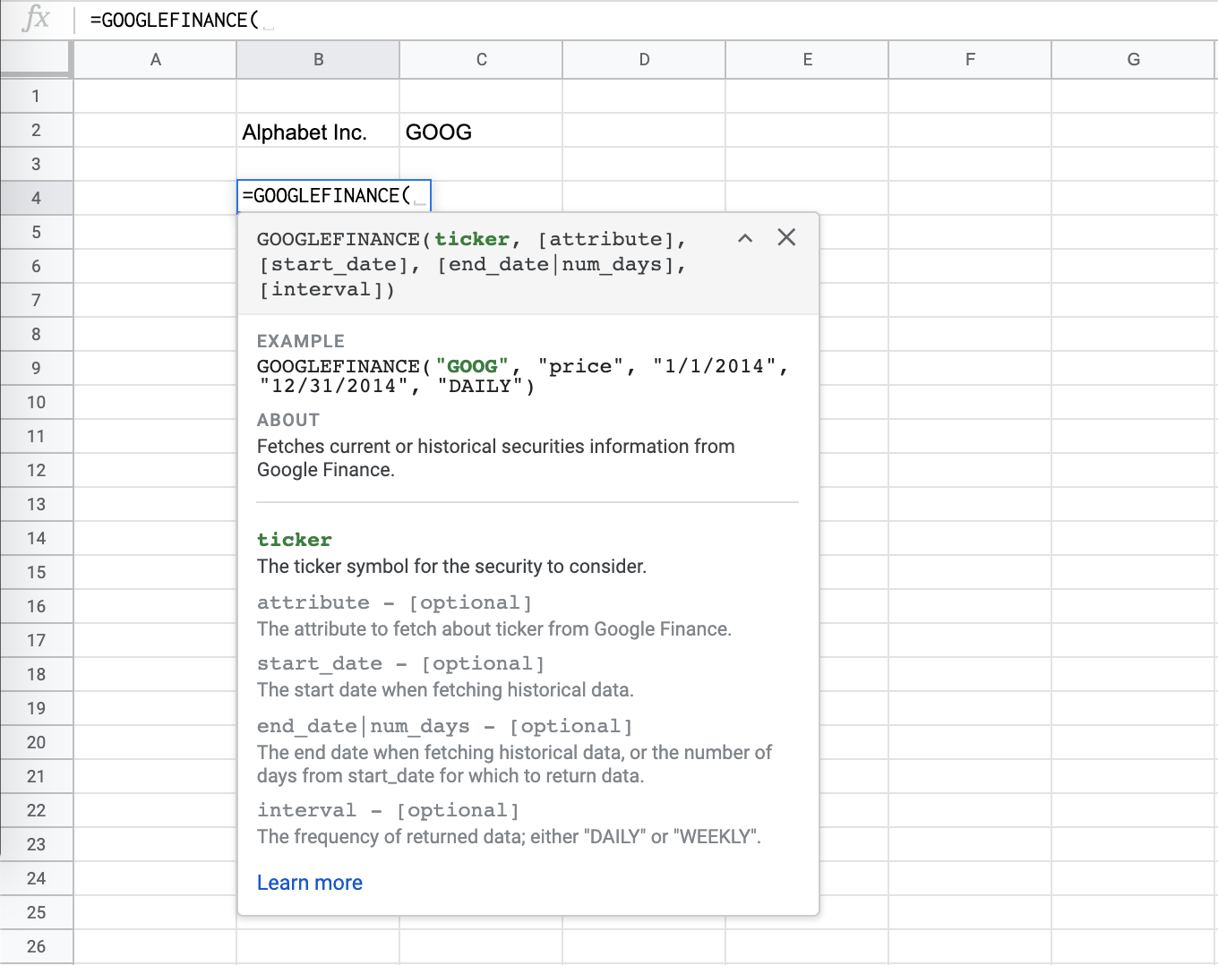
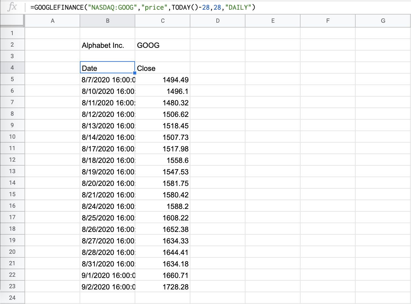
- Choose where you want your Google Finance data to populate. In this example, we picked cell B4. Type in the equal sign and our function, GOOGLEFINANCE.

- Read through the required inputs of the function.
- We want Alphabet Inc’s ticker symbol, “GOOG”. We want the information for the daily price for the past 28 days.
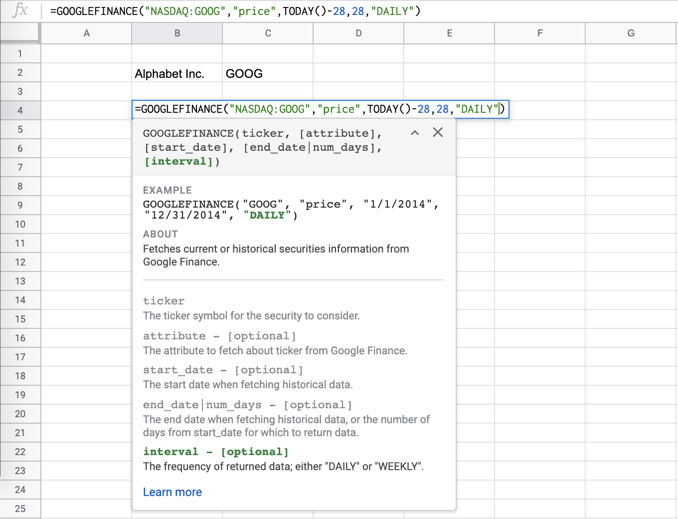
- Hit enter and the data should populate your sheets, with the proper headers. Note that there are only 19 entries. Google Finance omits any non-trading days from the set.
- Next, create another column for your Simple Moving Average. Input the AVERAGE function.

- Input the range, adding the previous 7 daily entries.

- Hit enter.
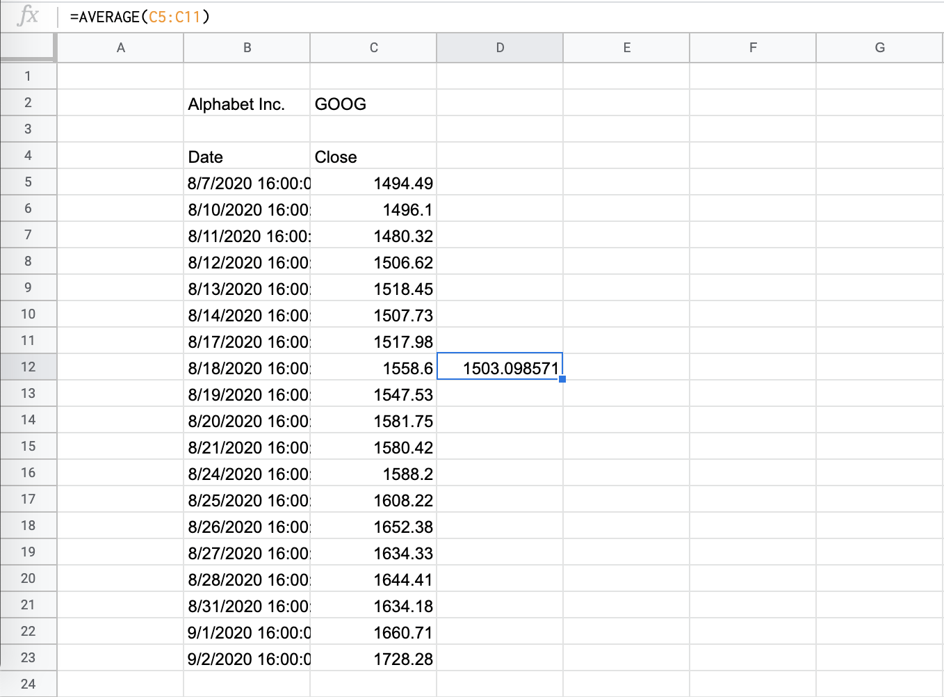
- Use the lower right handle to fill the rest of the column with the same formula. Note that the formula preserves the 7-day previous range.

- Ta-da, you’re done!

There you have it! You are now able to highlight a set of alternate rows in Google Sheets as you wish, without disturbing the integrity of your data. Now that you have a grasp on how to combine data visualization styles in your spreadsheets, you can combine this with other Google Sheets formulas to make really powerful data documents!


