The TEXTJOIN function in Google Sheets is useful if you want to concatenate or join values with a given delimiter.
Meaning, the function allows you to combine 2 or more string values with an option to put a delimiter between each value.
Table of Contents
The rules for using the TEXTJOIN function in Google Sheets are as follows:
- The number values passed to the TEXTJOIN function will be converted to text values during the process.
- The function returns a string/text value.
- There can be 252 text values that can be joined together.
Let’s take an example.
Reese would like to get the full name of each individual using the given data below:
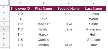
He can do it manually. However, he knows that, sooner or later, the number of employees would become more, and manually combining text values would be time-consuming and tedious.
So, he decided he might as well use a function to achieve his goal. Take a look at the table he worked on below:

Reese simply used the TEXTJOIN function with space ( ) as the separator for each text value.
Let’s have another example!
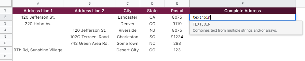
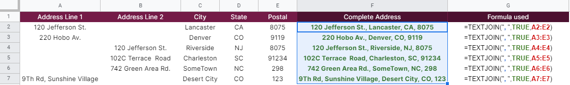
Ace is tasked to concatenate the columns Address Line 1, Address Line 2, City, State, and Postal Code to be able to create the Complete Address column.

Each text value should be separated by a comma (,).
He tried to use the CONCATENATE function. However, it provides a different result.
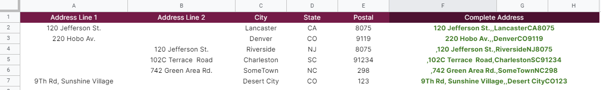
Why is this so?
Well, that’s because, unlike the TEXTJOIN function, the CONCATENATE function doesn’t have the option to deal with blank values. Hence, there were extra commas appeared in the results.

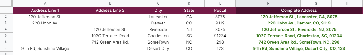
Ace used the TEXTJOIN instead. See how his table looks like:
Watch out for a more advanced tutorial and examples on how you can use the TEXTJOIN function in the coming weeks. Be sure to subscribe to be notified.
Perfect! Let’s begin getting to know more about our TEXTJOIN function in Google Sheets.
The Anatomy of the TEXTJOIN Function
So the syntax (the way we write) the TEXTJOIN function is as follows:
=TEXTJOIN( delimiter, ignore_empty, text1, [text2,...text_n] )
Let’s dissect this thing and understand what each of these terms means:
- = the equal sign is just how we start any function in Google Sheets. It is how Google Sheets understand that we are asking it to either do computation or use a function.
- TEXTJOIN() this is our TEXTJOIN function. It joins or combines the provided text values with or without a separator for each value.
- delimiter is a character or string placed between each text value in the resulting string. The most commonly used delimiters are space ( ) and comma (,).
- ignore_empty identifies whether empty values are included in the resulting string. TRUE ignores the empty value and FALSE includes the empty one.
- text1, text2, … text_n are the text values that you wish to combine or join together.
A Real Example of Using TEXTJOIN Function
Take a look at our names example below to see how the TEXTJOIN function is used in Google Sheets.

The resulting string in row 2, the full name ‘John Keith Ramos’, is achieved by joining the text values in columns B, C, and D.
Please note that the first argument in the TEXTJOIN function is a space enclosed with quotation marks. This resulted in joining the texts ‘John’, ‘Keith’, and ‘Ramos’ separated by space ( ).
We cannot remove the first argument to denote that we don’t want any delimiter between text values. This would cause a #N/A error.

Instead, we can remove the space in the first argument. Removing the space as the delimiter would result in the following:

The second argument used in the TEXTJOIN function is TRUE, which means empty values would be ignored. See our two examples below:
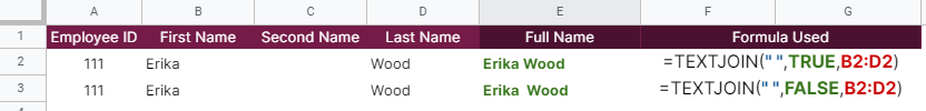
For the item in row 2, note that we passed TRUE as the second argument. Notice how it ignored the blank value in column C in the resulting string in column E. It shows only one space between the First Name and the Last Name.
On the other hand, notice the resulting string in column E for the item in row 3. Since we passed FALSE as the second argument in our TEXTJOIN function in row 3, two spaces are appearing between the First Name and the Last Name.

Why is this so?
The reason is that, since it didn’t ignore blank values, the resulting string included the blank value in column C for the item in row 3.
The two spaces between the First and Last names are the space ( ) from the delimiter and another space because of the blank value in column C.
Having TRUE as the second argument is advisable to use especially if there are blank values in the range or a list of text values to be joined together.
Lastly, our third argument in the TEXTJOIN function is simply the cell range where our text values to be combined are located.
You may make a copy of the spreadsheet using the link I have attached below.
How to Use TEXTJOIN Function in Google Sheets
- Click on any cell to make it the active cell. For this guide, I will be selecting F2, where I want to show the resulting string.

- Next, type the equal sign ‘=‘ to begin the function and then follow it with the name of the function, which is our ‘textjoin‘ (or ‘TEXTJOIN‘, not case sensitive like our other functions).
- Type open parenthesis ‘(‘ or simply hit Tab key to let you use that function

- Now the exciting part! Let’s give our function its first argument, the delimiter. In this example, we will be using the comma (,) and a space after as the delimiter. Type in quotation mark (“) and follow it with a comma (,) then space ( ) after. Don’t forget to end the delimiter with another quotation mark (“).

- To let the Google sheet know that we’re done typing our first argument, we should now type in the delimiter or the character that separates each argument on a function. In this case, type comma ‘,’.

- Type in our second argument, which is the ignore_empty. Type in TRUE (not case sensitive) and follow it with another comma (,).

- Lastly, we will now pass to the function the third argument, which is the list or range of text values to be joined together. Please note that you can type in the exact text values directly in our function. Just don’t forget to enclose them with quotation marks and separate them with commas. In this scenario, I will use the cell range where our text values are, which is A2 to E2. Simply type in A2:E2.

- Finally, hit your Enter or Tab key. Cell F2 will now show you the resulting string or the return value of the TEXTJOIN function.

- Copy the formula down to the remaining rows.
That’s pretty much it. You can now use the TEXTJOIN function in Google Sheets together with the other numerous Google Sheets formulas to create even more powerful formulas that can make your life much easier.