To merge duplicate rows in Google Sheets seems complicated to me.
There are times when I don’t really know when to merge, or is it useful, though?
But, as years passed by, I then realized the fact that Google Sheets wouldn’t have something that isn’t helpful. In that case, I thought of a scenario where merging can be utilized. That’s where I remembered that years ago, our school librarian had to sort lots of books and movie titles. This is where merging duplicate rows in Google Sheets is essential.
I made this guide not only for our librarians out there but also for the other users who feel the need to merge duplicate rows and the use of concatenate function.
Table of Contents
Let’s dive into a real example to understand better how to merge duplicate rows in Google Sheets.
Say we want to help Mrs. Brown, the librarian, sort all the books in ABC Library according to its genre. We are given this information:
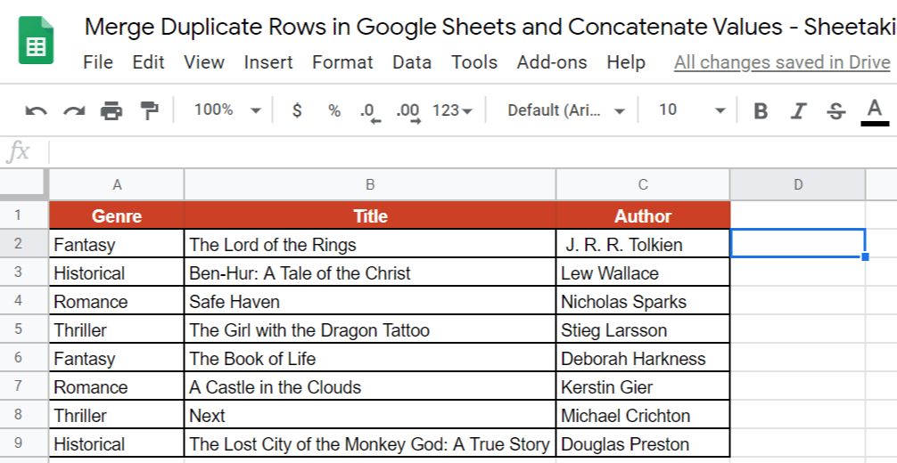
We will show you the four methods on how to merge duplicate rows in Google Sheets. We’ll then see if they provide the same output.
How to Merge Duplicate Rows in Google Sheets: 4 Ways
1. The Concatenate Values to Merge Duplicate Rows in Google Sheets
When we want to combine words and/or letters, we usually make use of an ampersand (&) sign instead of writing “and” many times. It’s like, peanut butter & jelly, R&R (for rest & relaxation), and even AT&T.
Same with Google Sheets, when we want to combine cells, we can use the ampersand (&), together with the CONCATENATE function.
Note that we can only use this method for small data. Meaning, you know where the specific positions are.
We have prepared two ways on how to concatenate values.
The first way is to merge cells with spaces between the values.
We can use either the ampersand (&) sign or the CONCATENATE function. We will discuss both below:
-
The Ampersand (&) Sign
Between the two, this is a little bit more complex, but we’ll make it easy for you. When adding a text string in any function in Google Sheets, we should enclose it in a quote-unquote symbol, just like this ~ “text here”. It has almost the same idea as in this method.
We wanted to sort the books according to their genre, and for this guide, we’ll have Fantasy as our example. By looking at the information given by Mrs. Brown, we can see that only cells B2 and B6 are classified as Fantasy. Therefore, we take them into the formula.
![]()
As you can observe, we didn’t add any function. Instead, we used the ampersand (&) sign. Notice that the quote-unquote (“”) symbol was kind of enclosed in the ampersand. This formula will give us this output:

-
The
CONCATENATEFunction
The CONCATENATE function allows us to combine cells with texts. To do this, we just have to add the strings needed to make this work nicely.
![]()
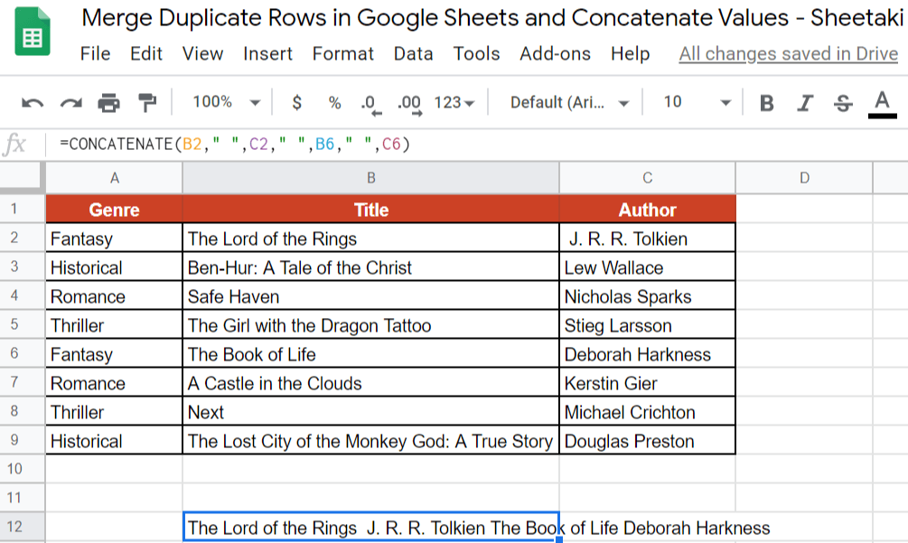
This formula above will give us the same output as the previous manner, but this is simpler. With the CONCATENATE function, you just have to supply the attributes such as the strings. as seen above.
The same thing. Since we are to merge the Fantasy books, then we just have to click on the cells that have Fantasy as a genre. In this case, rows 2 and 6 have it.
The second way to merge duplicate rows in Google Sheets under the concatenate values is to use spaces with any other marks to combine duplicate rows.
Yes, indeed, we could also make use of the ampersand (&) the CONCATENATE function. See how their outputs differ significantly from the previous ones:
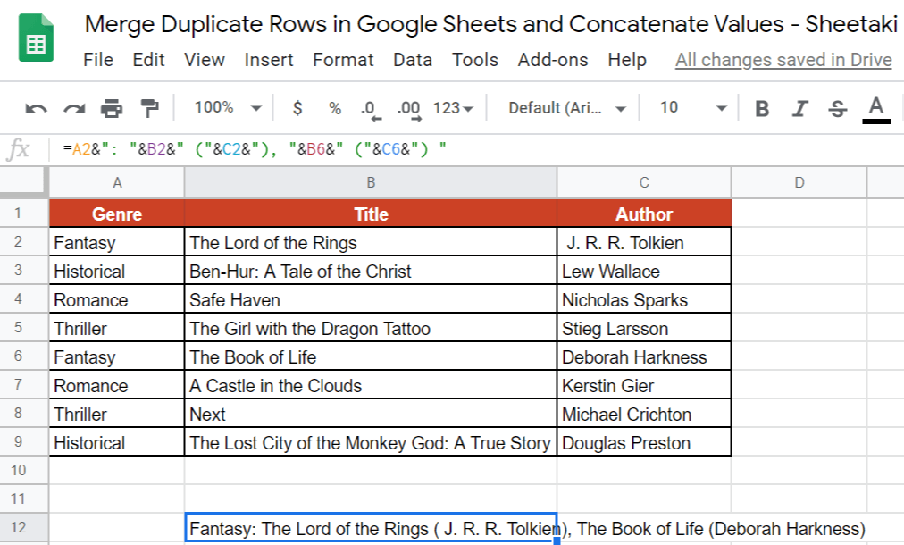

As you can observe, using any of these two, we came up with a format: Genre, then a colon (:) sign, followed by the two Fantasy books with the authors enclosed by a parenthesis.
2. Keeping Data with UNIQUE + JOIN to Merge Duplicate Rows in Google Sheets
Let’s dive a little deeper. The UNION and JOIN functions play an essential role. The UNIQUE function returns the list of unique items ~ in this case, the Genre. No matter how many times it is repeated, it will always give you a unique list.
On the other hand, the JOIN function combines values in one cell with a comma. We will also seek the help of the FILTER function, which would then be responsible for scanning all instances in a specific column.
Given the same example as above, we’ll show you how this is done:
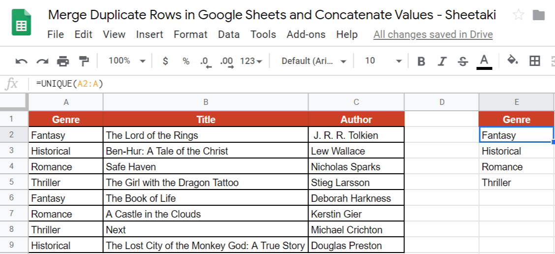
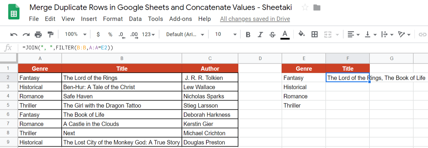
We selected cell E2 because this is where we want to start the list of book genres. We then used the UNIQUE function. Subsequently, we also chose the cell where our list would start, which will be cell A2 (this is up to you if you’re doing this yourself). Since we want to list down all the genre, then, we have to place the column where it is to be found. Therefore, we wrote A.
After the step above, we then moved forward by using the JOIN and FILTER functions. In the last part of our formula, we wrote E2, which is ‘Fantasy’. As you can see, it resulted in the book titles which are labeled as ‘Fantasy’.
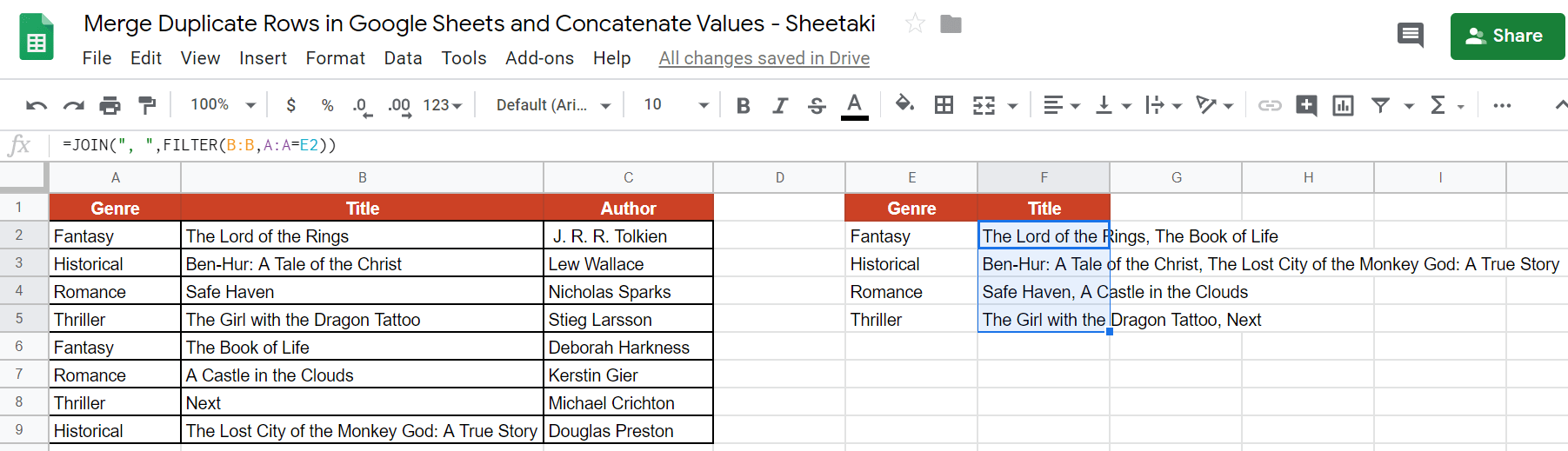
We dragged the formula down, and it automatically filled out the rest.
3. The QUERY Function to Remove Duplicate Rows
The QUERY function is essential, especially if we are working on a large data table. This function would simply identify the conditions given and immediately get the specific data based on the requirement. The QUERY function needs to have data, a set of commands (or the query), followed by the header/s. The header is optional.
Say we are sorting out thousands of books. Since it would be too time-consuming if we used the previous methods, this is where the QUERY function is handy. Just imagine out of thousands of books, we only have to find out which books are labeled as ‘Fantasy’. Using the QUERY function, it would then give us this output:

The formula, =QUERY(A1:C,"select * where A='Fantasy'"), tells that from ranges A1 to column C, the QUERY function should identify those books that are labeled as ‘Fantasy’ in column A.
As you hit on the ‘Enter’ key, all the ‘Fantasy’ books will automatically populate. Super easy, right?
4. The Use of Power Tools
This is the quickest way to merge duplicate rows in bulk. That is made possible using the Power Tools Add-on in Google Sheets. All you have to do is to install it by following the below steps:
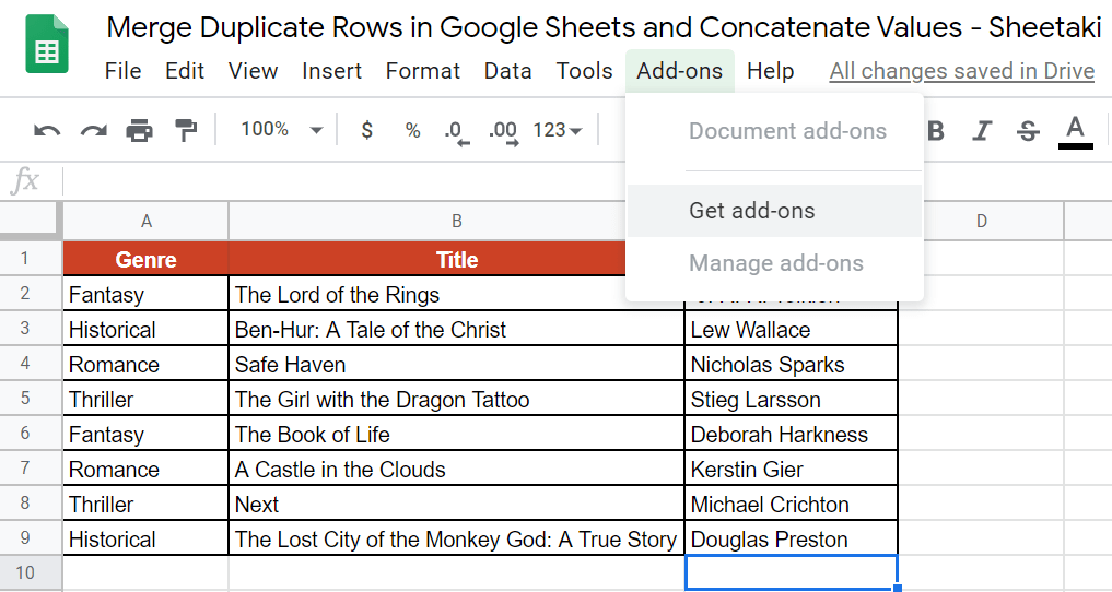


Let’s dive deeper into this Power Tools. As soon as the Power Tools is up and running, you may now navigate it to: Add-ons > Power Tools > Merge & Combine > Combine Duplicate Rows
So, I added a couple of duplicates from our original information. Also, I added the quantity. Say that we are trying to do an inventory.

The good thing about Power Tools aside from the fact that they work well with large data is that, in just three steps, we are already given the data we need, including all the SUMS and other functions that you may need.
Here’s what you do, step-by-step:
- Select the data range.
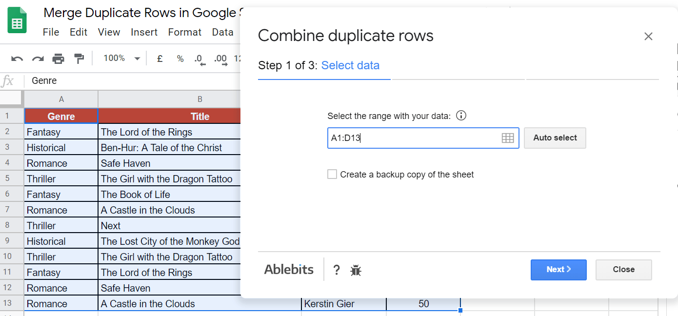
- Choose the key columns with duplicates.
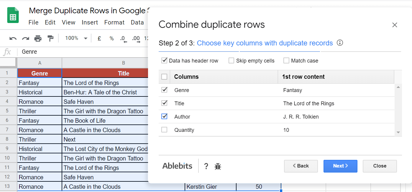
- Choose columns with the values to merge. At this step, you are allowed to modify the Action and Function based on what you need.
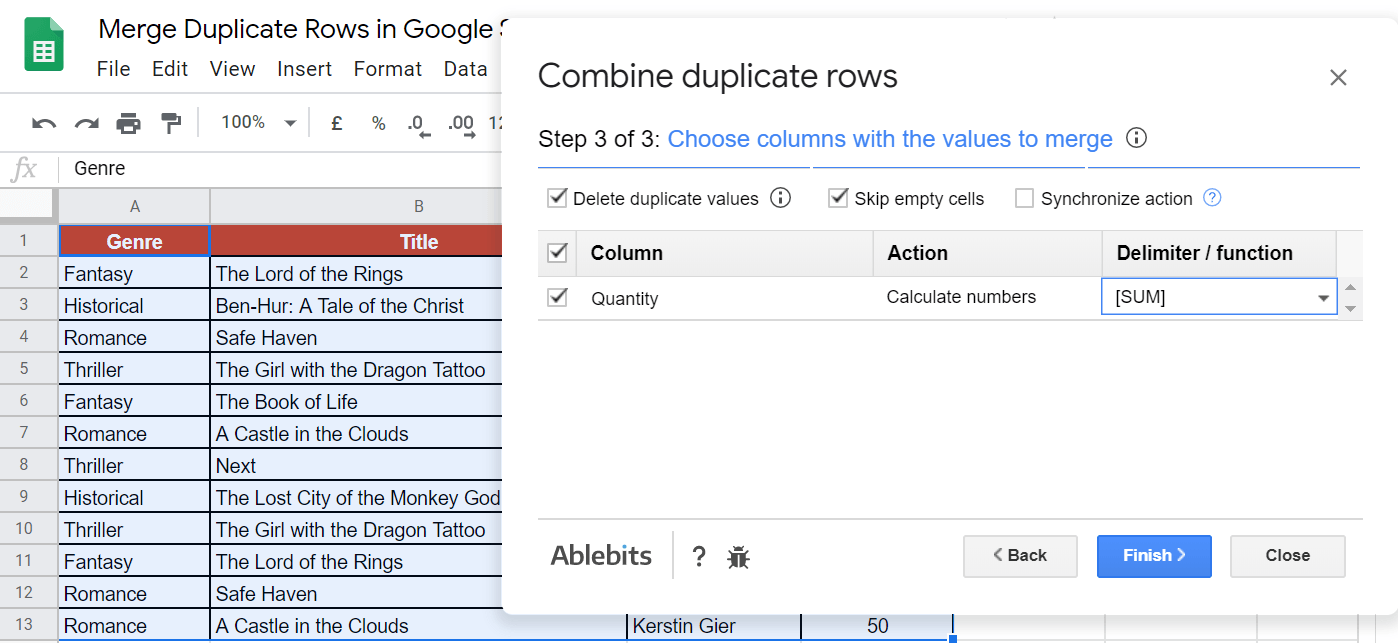
You’ll know that the Power Tools worked if it gave you this kind of summary:

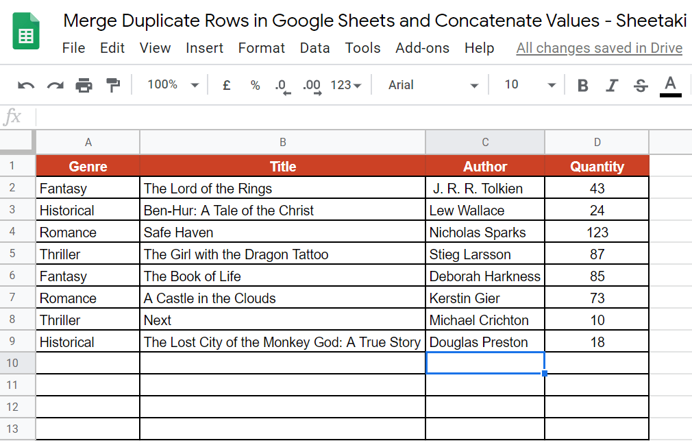
The final output when you use the Power Tools to merge duplicate rows is:
And that’s pretty much it! Now you know how to merge duplicate rows in Google Sheets. You may make a copy of the spreadsheet here: